The 3D Modeling of GATEM in Fractured Random Media Based on FDTD
Qiong Wu1, Yuehan Zhang1, Shanshan Guan1, Dongsheng Li1, and Yanju Ji1, 2*
1College of Electrical Engineering and Instrumentation
Jilin University, Changchun 130026, China
2Key Laboratory of Earth Information Detection Instruments
Ministry of Education, Jilin University, Changchun 130026, China
wuqiong_515@sina.cn, yhzhang19@mails.jlu.edu.cn, guanshanshan@jlu.edu.cn,
lidongsheng86@sina.cn, jiyj@jlu.edu.cn
Submitted On: March 18, 2021; Accepted On: July 30, 2021
Abstract
Grounded-source airborne time-domain electromagnetic (GATEM) method is an effective detection method of geological survey. The real geological media are rough, self-similar characteristics, and the diffusion process is anomalous diffusion. This paper primarily considers the GATEM responses of a grounded wire source in random media. Von Kármán function is used to establish three-dimensional (3D) random media model and the GATEM responses are realized based on 3D finite-difference time-domain (FDTD) method. The method is verified by homogeneous half-space model. The electromagnetic responses of random abnormal body model are analyzed, and the results show that the abnormal body can be clearly identified. The electromagnetic responses of a fractured model are analyzed, and the results show that the tilt angle of the fault can be reflected.
Index Terms: FDTD, GATEM, Hurst exponent, random media.
I. INTRODUCTION
In recent years, there is a new kind of airborne electromagnetic method appearing on the international aviation, grounded-source airborne time-domain electromagnetic (GATEM) method, which is suitable for the large area where is difficult to access [1]. GATEM takes the form of a grounded wire transmitter and the receiver carried by aircraft [2]. It gathers large investigation depth of ground electromagnetic method and high efficiency of airborne electromagnetic method. It has been used in engineering, geological surveying, and mineral exploration [3, 4, 5].
The electromagnetic modeling of subsurface media is usually based on usually homogeneous media [5, 6, 7, 8]. However, many geophysicists realize that electromagnetic induction of subsurface media is anomalous diffusion [9, 10, 11]. The mean-square displacement of subdiffusion process is slower (subdiffusion) or faster (superdiffusion) than that of Gauss diffusion process, and it is proportional to the fractional power of time [12]. This paper primarily focuses on the subdiffusion diffusion. For subdiffusion diffusion, the electromagnetic fractional diffusion model is defined and the fractional Maxwell equations are gradually being promoted [13, 14, 15]. The three-dimensional (3D) finite-difference (FD) of controlled-source electromagnetics (CSEM) is proposed in frequency domain for a multiscale random media model of fractured geologic formation which is based on a von Kármán autocorrelation function [16]. The one-dimensional (1D) GATEM modeling and interpretation method of fractional diffusion model for a rough medium is proposed [17].
In this paper, we mainly aim to obtain 3D time-domain response of a grounded wire source in fractured media. For the fractional diffusion model based on a von Kármán autocorrelation function, the electromagnetic field iterative equations are derived based on finite-difference time-domain (FDTD) method. The modeling method is validated by different models and compared with analytical solutions.
II. METHOD
A. 3D fractured random media model
The random media conductivity model of geologic formation can be expressed as [16, 18]:
| (1) |
where is the usual dimension of the conductor, is the smaller scale random inhomogeneities.
The 3D computational model is divided by using Yee staggered grids. The autocorrelation function related to the grid step based on isotropic von Kármán function is:
| (2) |
where v represents roughness or Hurst exponent and 0v1, a is the correlation length, , (v) represents the gamma function, and K represents the Bessel function of the second kind of noninteger order.
The square root of the autocorrelation spectrum f(C(r)) and Fourier transform of a white noise field wn are calculated and multiplied in the wavenumber domain. The is obtained by transforming results to the spatial domain. The smaller scale random inhomogeneities is added to to obtain the random media conductivity .
B. Modeling of GATEM in fractured random media model
The fractional Maxwell equations are:
| (3) |
| (4) |
where E(t) is the electric field, H(t) is the magnetic field, and are the magnetic permeability and permittivity, respectively.
It is necessary to subdivide the model, when calculating the GATEM response of a 3D anomalous body based on FDTD. In this paper, a non-uniform grid is used to calculate the GATEM response, as shown in Figure 1 (a). The mesh of a part area is relatively finely divided according to the needs, and the mesh of other areas is coarsely divided. The electric field is sampled at the edge of the Yee cell, and the magnetic field is sampled at the center of the Yee cell’s face [19]. According to Figure 1 (b), the electric field is surrounded by four magnetic fields, and the magnetic field is surrounded by four electric fields.
The electric field iterative formulation based on FDTD is:
| (5) |
where is the electric field of t at position , y and z are space step. t is the time step, and the initial moment is
| (6) |
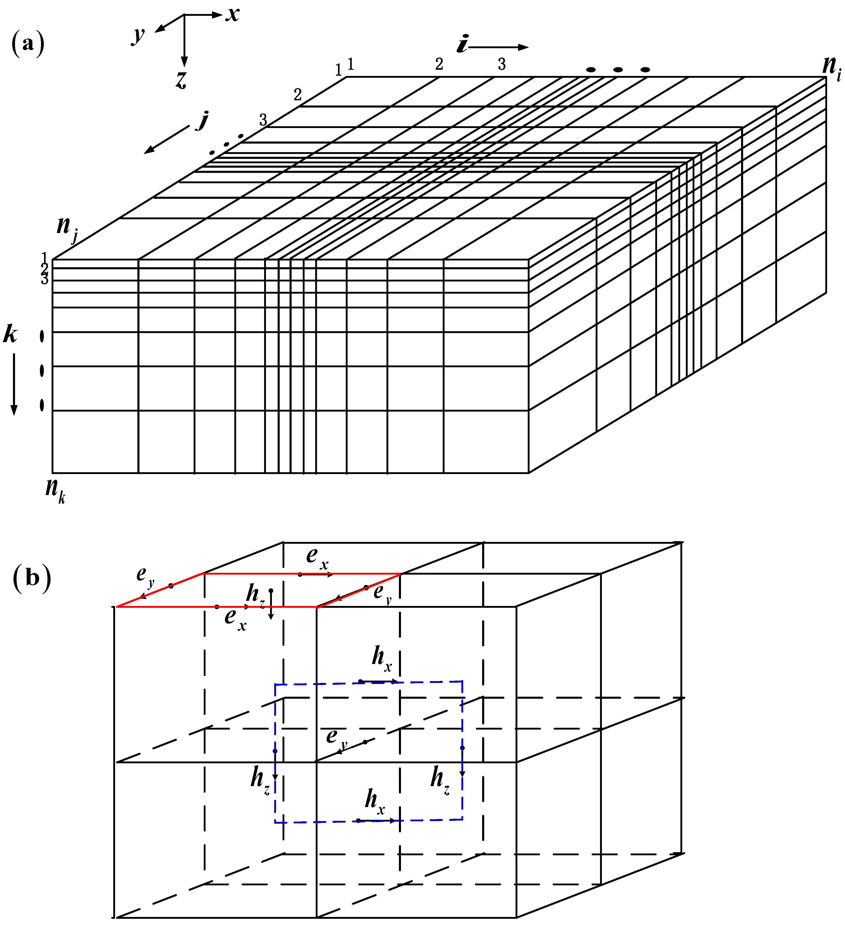
Fig. 1. (a) non-uniform grid, (b) Electric field and magnetic field at Yee’s cell.
where is the electrical conductivity of top grid and is the top grid. In FDTD, to ensure the stability of calculation, it is necessary to follow Courant–Friedrichs–Lewy stability conditions. In practice, the maximum time step is [20]
| (7) |
where ranges from 0.1 to 0.2, and is the minimum resistivity value in the model, is the minimum grid spacing. For the magnetic fields, according to control equations, the iterative formulation is
| (8) |
when t = nt,
| (9) |
For the GATEM system, the transmitter is a grounded electric source with several kilometres length wire, and the receiver and induction coil are towed by an aircraft in the air. For 3D modeling of GATEM based on FDTD, the initial condition of calculation is the electromagnetic response of a grounded wire source. When t = t, the electric fields of the grounded wire placed along the x-axis are
| (10) |
| (11) |
where , , ,, , L is the half length of the ground wire, I is the transmitter current, u = in quasistatic electromagnetic field, is the Hankel transform integral variable, r is the reflection coefficient, and J is the first-order Bessel function. The Bessel function integral is calculated via the Hankel transformation algorithm [21]. The time domain responses can be converted from frequency domain by digital filtering method [22].
III. RESULTS
A. The fractured random media conductivity model
Figure 2 is the conductivity distributions of fractured random media conductivity model. The correlation length a = 10 and the conductor is 0.1 Sm. The Hurst exponent v set as 0.2, 0.5, and 0.8. The conductivities are 0.1 Sm to 0.145 Sm for v = 0.2, 0.1 Sm to 0.24 Sm for v = 0.5, and 0.1 Sm to 0.4 Sm for v = 0.8; the maximum value of conductivities increased by more than four times. The Hurst exponent v is an important parameter that determines the change of conductivity.

Fig. 2. Conductivity distribution of random media for Hurst exponent. (a) v = 0.2, (b) v = 0.5, (c) v = 0.8.
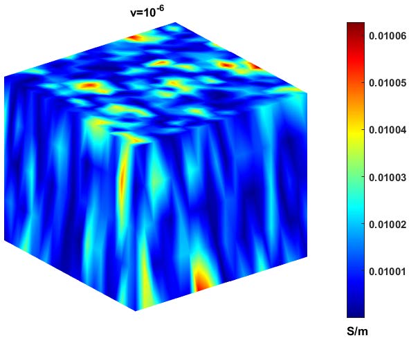
Fig. 3. Conductivity distribution of random media for roughness exponent v =10.
B. Modeling results
To validate the 3D modeling method, the GATEM response of a specific random half-space model which v 0, the limit as v 0 corresponds to a homogeneous medium, is calculated and compared with analytical solution. The Hurst exponent v = 10, and the conductor is 0.01 Sm. The conductivity distributions of random abnormal body are shown in Figure 3. The conductivities are almost 0.01 Sm, and it can be approximated as a homogeneous medium model. The calculation parameters are as follows: all models have 22122175 grids. The grid is non-uniform and the smallest spacing is 10 m, the largest spacing is 120 m. The wire source is located at the center of the model with 1 m length, and the transmitter current is 20 A. The receiver coil is 500 m away from the wire source and the height is 0 m. The GATEM response is calculated as shown in Figure 4.

Fig. 4. Comparison of GATEM response in a random half-space model when v = 10and analytical solution.
The GATEM response is compared with the analytical solution obtained from equation (12) [23]. The induced voltage (Vz) can be obtained from , where S is the equivalent area of receiver coil. The modeling result coincides with the analytical solution. Figure 4 validates the correctness of the modeling method. The relative error is calculated and is less than 8%.
| (12) |
where ds is the dipole length, r is the source–receiver distance, y is the horizontal transverse offset and = ()r.
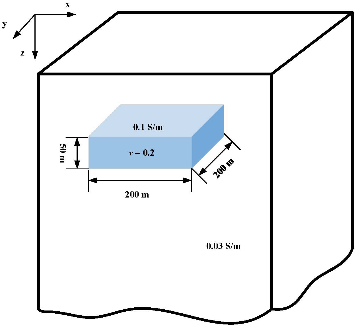
Fig. 5. A theoretical random abnormal body model.
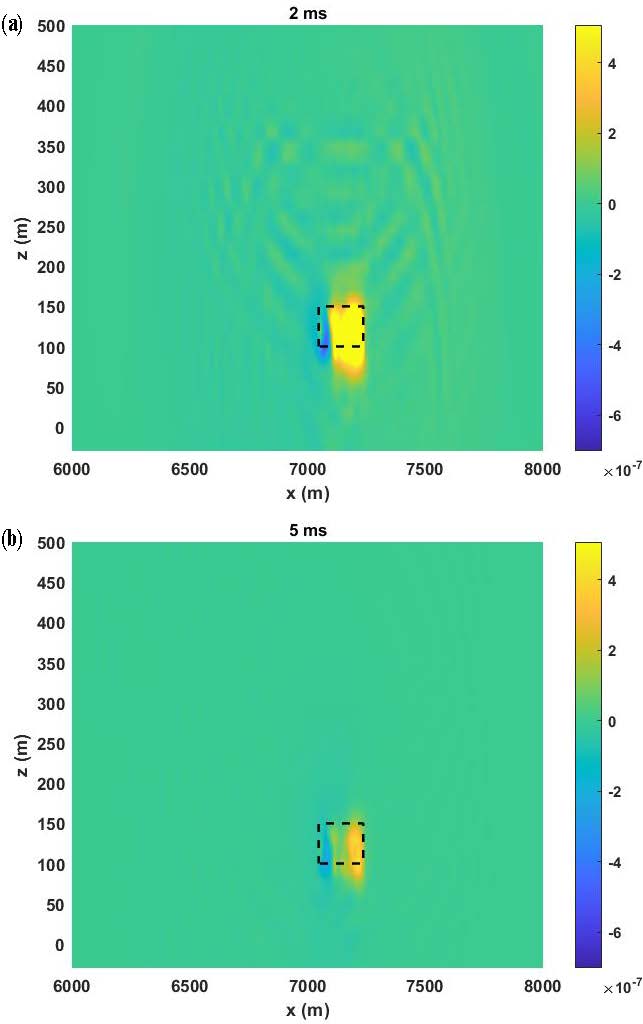
Fig. 6. The electromagnetic response slices of abnormal body model in x-z plane at 2 ms and 5 ms. The black dashed line is the position of the random abnormal body.

Fig. 7. The 3D fractured model.
Figure 5 is a 3D theoretical random abnormal body model and the center of the long wire source is the origin. The conductivity of bedrock is recorded as 0.03 Sm, and the conductivity of random abnormal body is variable and the basic conductivity is 0.1 Sm. The Hurst exponent is set as v = 0.2 and the conductivity distributions of random abnormal body is shown in Figure 1 (b). The depth of the abnormal body is 100 m and the size is 200 m 200 m 50 m. The electromagnetic response slices of abnormal body model with v = 0.2 in x-z plane at 2 ms and 5 ms are shown in Figure 6. From these slices in Figure 6, the responses can well reflect the information of the random abnormal body.
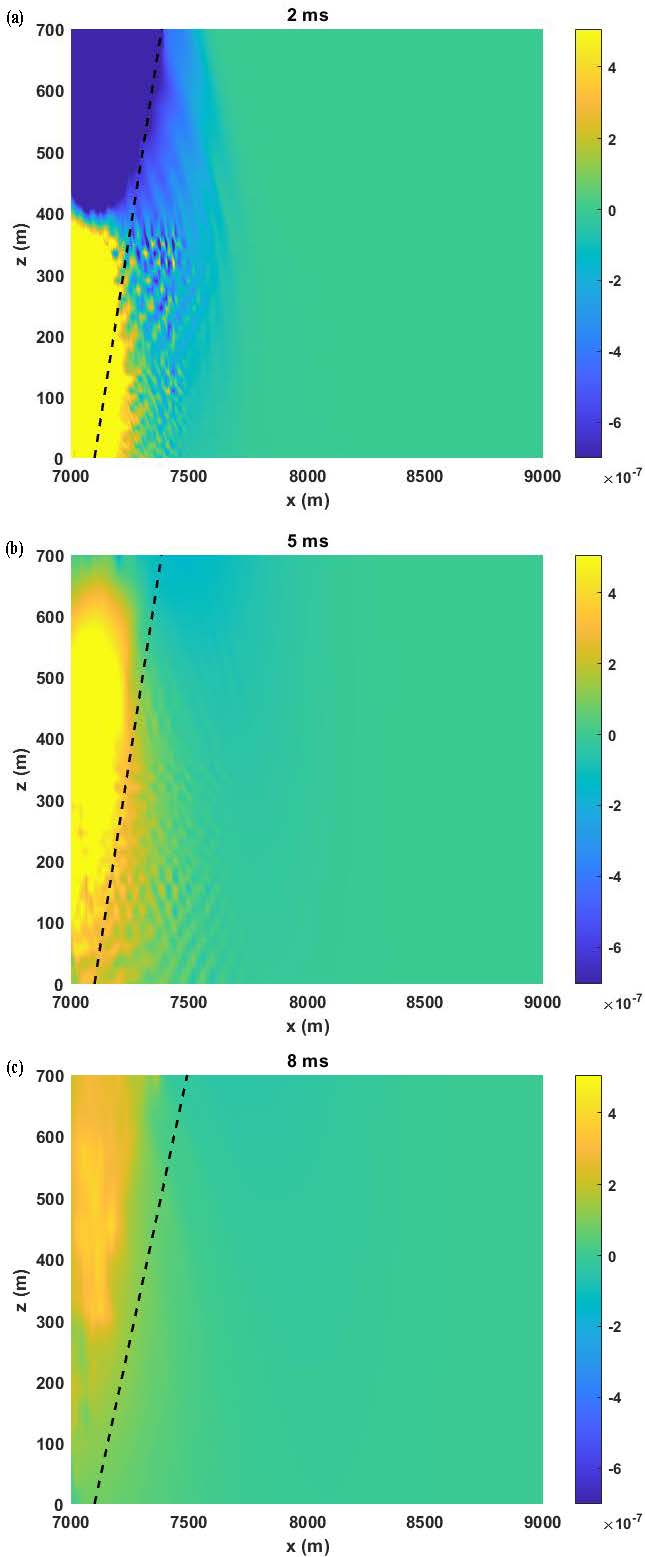
Fig. 8. The electromagnetic response slices in x-z plane at 2 ms, 5 ms, and 8 ms. The black dashed line is only the reference.
A 3D fractured model is designed, as shown in Figure 7. The resistivity of the right area is 0.03 Sm as the back ground. The basic conductivity of the left part changes linearly from 0.03 Sm to 0.1 Sm, and the Hurst exponent is v = 0.5, therefore, the conductivity is variable, ranging from 0.03 to 0.2 Sm. The electromagnetic response slices in x-z plane at 2 ms, 5 ms, and 8 ms are shown in Figure 8. It can reflect the tilt angle of the fault.
IV. CONCLUSION
In this paper, 3D random media model is established by Von Kármán function. When establishing a random media model, Hurst exponent is an important parameter that determines the change in conductivity. The GATEM responses in random media are realized based on FDTD and the modeling results validated correctness. The results of the random abnormal body model show that the abnormal body can be identified. A fractured model is designed and the results show that the tilt angle of the fault can be reflected. Inversion of the 3D modeling for random media is the focus of our following research.
ACKNOWLEDGMENT
This study was performed under the project entitled “Research on Sub-diffusion Multi-parameter extraction method of Ground-source Airborne Electromagnetic data based on fully connected neural network (42004059)” and “Research on Key Technologies of Electromagnetic Detection of Induction-Polarization Symbiosis Effects of Dual Phase Conductive Medium Based on SQUID technique (42030104)” supported by the National Natural Science Foundation of China. We thank all members of the GATEM group of Jilin University (China) for their support of this study.
REFERENCES
[1] R. S. Smith, A. P. Annan, and P. D. McGowan, “A comparison of data from airborne, semi-airborne, and ground electromagnetic systems,” Geophysics, vol. 66, no. 5, pp. 1379-1385, Oct. 2001.
[2] T. Mogi, Y. Tanaka, K. Kusunoki, T. Morikawa, and N. Jomori, “Development of grounded electrical source airborne transient EM (GREATEM),” Exploration Geophysics (Melbourne), vol. 29, no. 2, pp. 61-64, Jun. 1998.
[3] T. Mogi, K. Kusunoki, H. Kaieda, H. Ito, A. Jomori, N. Jomori, and Y. Yuuki, “Grounded electrical-source airborne transient electromagnetic (GREATEM) survey of Mount Bandai, north-eastern Japan,” Exploration Geophysics, vol. 40, no. 1, pp. 1-7, Feb. 2009.
[4] S. A. Allah, T. Mogi, H. Ito, A. Jymori, Y. Yuuki, E. Fomenko, K. Kiho, H. Kaieda, K. Suzuki, and K. Tsukuda, “Three-dimensional resistivity modelling of grounded electrical-source airborne transient electromagnetic (GREATEM) survey data from the Nojima fault, Awaji island, south-east Japan,” Exploration Geophysics, vol. 45, no. 1, pp. 49-61, Dec. 2014.
[5] Y. Ji, Y. Zhu, M. Yu, D. Li, and S. Guan, “Calculation and application of full-wave airborne transient electromagnetic data in electromagnetic detection,” Journal of Central South University, vol. 26, no. 4, pp. 1011-1020, Apr. 2019.
[6] Y. Shao and S. Wang, “Truncation error analysis of a pre-asymptotic higher-order finite difference scheme for maxwell’s equations,” Applied Computational Electromagnetics Society Journal, vol. 30, no. 2, pp. 167-170, Feb. 2015.
[7] M. Commer, P. V. Petrov, and G.A. Newman, “FDTD modelling of induced polarization phenomena in transient electromagnetics,” Geophysical Journal International, vol. 209, no. 1, pp. 387-405, Apr. 2017.
[8] F. Naixing, Y. Zhang, Q. Sun, J. Zhu, W. T. Joines, and Q. H. Liu, “An accurate 3-D CFS-PML based Crank-Nicolson FDTD method and its applications in low-frequency subsurface sensing,” IEEE Transactions on Antennas and Propagation, vol. 66, no. 6, pp. 2967-2975, Jun. 2018.
[9] B. Berkowitz and H. Scher, “Anomalous transport in random fracture networks,” Physical Review Letters, vol. 79, no. 20, pp. 4038-4041, Nov. 1997.
[10] A. Guellab and W. Qun, “High-order staggered finite difference time domain method for dispersive debye medium (Artical),” Applied Computational Electromagnetics Society Journal, vol. 33, no. 4, pp. 430-437, Apr. 2018.
[11] C. J. Weiss, B. G. van Bloemen Waanders, and H. Antil , “Fractional operators applied to geophysical electromagnetics,” Geophysical Journal International, vol. 220, no. 2, pp. 1242-1259, Feb. 2020.
[12] R. Metzler and J. Klafter, “The random walk’s guide to anomalous diffusion: a fractional dynamics approach,” Physics Reports: A Review Section of Physics Letters (Section C), vol. 339, no. 1, pp. 1-77, Dec. 2000.
[13] M. E. Everett, “Transient electromagnetic response of a loop source over a rough geological medium,” Geophysical Journal International, vol. 177, no. 2, pp. 421-429, May 2009.
[14] J. Ge, M. E. Everett, and C. J. Weiss, “Fractional diffusion analysis of the electromagnetic field in fractured media; Part I, 2D approach,” Geophysics, vol. 77, no. 4, pp. WB213-WB218, Jul. 2012.
[15] X. Zhao, S. Wang, Q. Wu, and Y. Ji, “Time-domain electromagnetic fractional anomalous diffusion over a rough medium,” IEEE Transactions on Antennas and Propagation, pp. 1-1, Dec. 2020.
[16] J. Ge, M. E. Everett, and C. J. Weiss, “Fractional diffusion analysis of the electromagnetic field in fractured media; Part 2, 3D approach,” Geophysics, vol. 80, no. 3, pp. E175-E185, May 2015.
[17] Q. Wu, D. S. Li, C. D. Jiang, Y. J. Ji, Y. L. Wen, and H. Luan, “Ground-source Airborne Time-domain ElectroMagnetic (GATEM) modelling and interpretation method for a rough medium based on fractional diffusion,” Geophysical Journal International, vol. 217, no. 3, pp. 1915-1928, Jun. 2019.
[18] L. Klimeš, “Correlation functions of random media,” Pure and Applied Geophysics, vol. 159, no. 7, pp. 1811-1831, Jul. 2002.
[19] Kane Yee, “Numerical solution of initial boundary value problems involving Maxwell’s equations in isotropic media,” IEEE Transactions on Antennas and Propagation, vol. 14, no. 3, pp. 302-307, May 1966.
[20] T. Wang and G. W. Hohmanni, “A finite-difference, time-domain solution for three-dimensional electromagnetic modeling,” Geophysics, vol. 58, no. 6, pp.797-809, Jun. 1993.
[21] F. N. Kong, “Hankel transform filters for dipole antenna radiation in a conductive medium,” Geophysical Prospecting, vol. 55, no. 1, pp. 83-89, Jan. 2007.
[22] D. Guptasarma, “Computation of the time-domain response of a polarizable ground,” Geophysics, vol. 47, no. 11, pp. 1574-1576, Nov. 1982.
[23] M. N. Nabighian, “Electromagnetic methods in applied geophysics, volume 1 theory,” Tulsa, Society of Exploration Geophysicists, pp. 237, Jan. 1988.
ACES JOURNAL, Vol. 36, No. 11, 1401–1406.
doi: 10.13052/2021.ACES.J.361102
© 2021 River Publishers