Convergence Determination of EMC Uncertainty Simulation Based on the Improved Mean Equivalent Area Method
Jinjun Bai1, Jingchao Sun2, and Ning Wang1
1College of Marine Electrical Engineering
Dalian Maritime University, Dalian, 116026, China
E-mail: baijinjun@dlmu.edu.cn, n.wang@ieee.org
2Traction & Control State Key Lab
CRRC Dalian R&D Co., Ltd, Dalian, 116052, China
sunjingchaofirst@126.com
Submitted On: April 2, 2021; Accepted On: July 29, 2021
Abstract
Uncertainty analysis plays a significant role in electromagnetic compatibility (EMC) simulation, but suffers from convergence determination thereby reducing simulation accuracy and computational efficiency. In this paper, an improved mean equivalent area method is proposed to enhance calculation accuracy. It shows that, using a benchmark example, the proposed method successfully achieves the convergence determination of the stochastic reduced order models (SROMs), and realizes further promotion of uncertainty analysis method.
Index Terms: EMC simulation, uncertainty analysis, convergence determination, improved mean equivalent area method, stochastic reduced order models.
I. INTRODUCTION
In order to accurately describe the randomness and the uncertainty in the actual engineering environment, the uncertainty simulation methods have received extensive attention in the field of electromagnetic compatibility (EMC) in recent years [1].
Among the uncertainty analysis methods, the Monte Carlo method (MCM) is the most commonly used. The MCM uses a large number of sampling points to simulate the randomness of the simulation input, and deterministic EMC simulation is performed at each sampling point to obtain the uncertainty analysis results [2, 3, 4]. However, the computational efficiency of the MCM is extremely low, which makes it gradually lose competitiveness.
Since 2013, the stochastic Galerkin method (SGM) and the stochastic collocation method (SCM) of the generalized polynomial chaos theory have been successfully applied in EMC simulation. They use chaotic polynomials under a specific order to expand the uncertainty output, and then obtain the uncertainty analysis results through the Galerkin projection technology or the multidimensional Lagrange interpolation technology [5, 6, 7, 8]. It is proved that the calculation accuracy of the SGM and the SCM is at the same level as the MCM, but their calculation efficiency is significantly higher than the MCM. However, when the number of random variables increases, the calculation time of the SGM and the SCM will increase exponentially, which is the so-called “dimension disaster” problem.
In 2016, the stochastic reduced order models (SROMs) have been proposed, which can completely avoid the emergence of the “dimension disaster” problem. Using the optimized algorithm for clustering, the SROM can select several feature points to represent sampling points under large number. Deterministic EMC simulation at each feature point is performed, and the final uncertainty analysis results can be obtained. The limitation of the SROM is that there is no way to judge whether the algorithm has converged, so the exact number of feature points cannot be determined [9].
In fact, for each uncertainty analysis method, how to accurately judge its convergence is a key issue that needs to be solved urgently. In other words, judging convergence is an indispensable step to determine the number of sampling points of the MCM, the order of chaotic polynomials of the SGM and the SCM, or the number of feature points of the SROM. Obviously, if the algorithm does not converge, there will be errors in the uncertainty analysis results. On the contrary, if an excessively large number of sampling points, chaotic polynomial orders or feature points are used in order to ensure convergence, it will be a waste of computing resources.
In order to solve the convergence determination problem of uncertainty simulation, the mean equivalent area method (MEAM) is proposed [10]. The MEAM draws on the idea of effectiveness evaluation in the feature selective validation (FSV) method, and applies the common area between the probability density curves of standard data and simulation data as the evaluation criterion. The effectiveness of the simulation results under adjacent orders or adjacent points is evaluated. When the evaluation result is “excellent” (the common area is greater than 0.95), it indicates that the algorithm has converged.
However, in order to achieve the purpose of standardization and generalization, the conventional MEAM uses a uniform distribution curve to replace the original probability density curve. Therefore, many details are ignored in calculating the common area, which reduces the accuracy of the algorithm.
This paper proposes the improved mean equivalent area method (Improved MEAM), which can accurately calculate the common area under the premise of ensuring standardization and generalization. Meanwhile, a convergence determination method based on the proposed method is given for the SROM, in order to determine the number of feature points.
The structure of this paper is as follows. The detailed description of the improved MEAM is provided in Section II. Section III offers the calculation accuracy verification of the improved MEAM. The convergence determination of the SROM is shown in Section IV. Discussion about convergence determination method of MCM, SGM, and SCM is given in Section V. Section VI presents the conclusion part of this paper.
II. IMPROVED MEAN EQUIVALENT AREA METHOD
Uncertainty analysis results are usually presented in the form of sampling points. Applying the statistical calculation, the expected value, the standard deviation, the worst-case estimate, or the probability density curve can be obtained. Obviously, the probability density curve is the most important result, because it can retain all the information of the uncertainty analysis. According to this feature, the conventional MEAM quantifies the difference between the simulation result and standard data by calculating the value of the common area surrounded by their probability density curves, in order to judge the accuracy of the simulation result. At the same time, in order to meet the needs of standardization and scalability, the conventional MEAM uses a uniform distribution curve to approximate the original probability density curve, and converts the calculation of the common area into the calculation of the rectangular area. This approximation ignores some details of the original PDF curve, which will bring calculation errors.
In the improved MEAM, N rectangles are used to approximate the probability density curve, aiming to ensure that the premise of standardization preserves the details of the probability density curve as much as possible, as shown in Figure 1. The specific steps of the approximate process are as follows:
1. Calculate the maximum value and the minimum value of M sampling points.
2. Take N–1 points at equal intervals between and to form N intervals, for example, N = 5 in Figure 1.
3. Count the number of sampling points in each interval M, and calculate the percentage.
4. Each rectangle is regarded as a uniform distribution with a total probability of .

Fig. 1. Approximation of probability density curve.
Both standard data and simulation results can be transformed into N rectangles, as shown in Figure 2. The calculation of the common area between the probability density curves is transformed into the calculation of the common area between the rectangles. According to reference [10], conventional MEAM can calculate the common area of two rectangles, so the common area calculation of the improved MEAM can be given by the following formula:
| (1) |
where represents the ith rectangle of the standard data, and represents the jth rectangle of the simulation result. indicates that the common area of two rectangles is calculated using the conventional MEAM, its calculation formula is as follows:
| (2) |
where represents the bottom of the rectangular common area, and is the height of the rectangular common area. The calculation formula for the height is:
| (3) |
where is the standard deviation of the uniform distribution represented by , and is the standard deviation of the uniform distribution represented by .
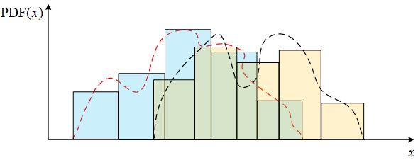
Fig. 2. The common area in the improved MEAM.
The bottom is determined by Table 1. The intermediate coefficient expression is:
| (4) |
where is the average value of the uniform distribution represented by , and is the average value of the uniform distribution represented by .
Table 1: Calculation results of
| Condition | ||
| 1 | 0 | |
| 2 | ||
| 3 | ||
| 4 | ||
| 5 | ||
| 6 | 0 |
Obviously, times conventional MEAM operations are required in one improved MEAM operation.
III. ACCURACY VERIFICATION OF THE IMPROVED MEAN EQUIVALENT AREA METHOD
In order to verify the accuracy of the improved MEAM, a calculation example of the common area problem is given. In calculation example, the probability density function of standard data is supposed as:
| (5) |
The probability density function of the simulation result is given as:
| (6) |
where the value of k can be changed to generate different calculation examples. In this section, the value of k ranges from 0.02 to 1.5, and sampling points are taken every 0.02, for a total of 75 examples. Figure 3 shows the calculation example when k is 0.2.
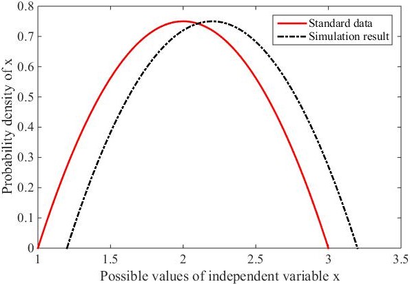
Fig. 3. Calculation example when k is 0.2.
It is worth noting that since the simulation result and the standard data are in the form of definite probability density functions, the real common area value can be obtained by directly performing integral operations.
In order to apply the conventional MEAM and the improved MEAM, the probability density function needs to be converted into the form of sampling points. Take the simulation result as an example, the distribution function is calculated first, which is shown as:
| (7) |
After sampling the interval according to the uniform distribution, the following equation can be solved:
| (8) |
The set of solution results becomes the sampling points that characterize the probability density function. Similarly, eqn. (5) can also be transformed into the form of sampling points.
Using the conventional MEAM and the improved MEAM to calculate the common area of 75 examples, the results are shown in Figure 4. Among them, the black solid line represents the standard data, and the result is obtained by integrating the probability density function. The blue dashed line is the calculation result of the conventional MEAM, and the red dashed line is the calculation result of the improved MEAM.
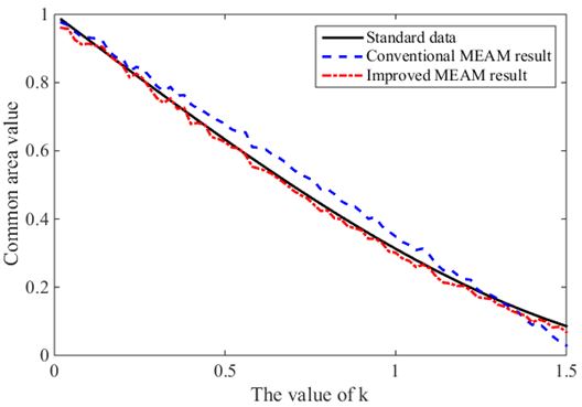
Fig. 4. Accuracy comparison of the conventional MEAM and the improved MEAM.
Compared with standard data, Figure 5 shows the calculation errors of the conventional MEAM and the improved MEAM respectively.
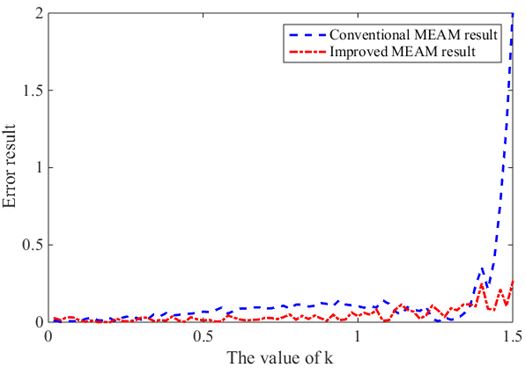
Fig. 5. Error results of the conventional MEAM and the improved MEAM.
Through calculation, the average error of the conventional MEAM is 12.94%, and that of the improved MEAM is 4.48%. Therefore, it is clearly proved that the proposed method has a greater improvement in the accuracy of calculating the common area than the conventional MEAM.
IV. CONVERGENCE DETERMINATION OF THE SROM
In this section, the improved MEAM is applied to judge the convergence of SROM, which is a popular uncertainty analysis method. The convergence decision criterion is as follows:
1. SROM is used to calculate the uncertainty analysis results when the number of feature points is 2 and , and the common area value of the two results is obtained through the improved MEAM. If the area value is greater than 0.95, go to step 3., otherwise go to step 2.
2. SROM is applied to continue to calculate the uncertainty analysis result when the number of feature points is , and calculate the common area value when the feature points are and . If it is greater than 0.95, enter step 3., otherwise continue to calculate the uncertainty analysis result when the number of feature points is , until the common area value is greater than 0.95 when the feature points are and .
3. When the number of feature points is , the algorithm is judged to be convergent. Its corresponding uncertainty analysis result is the result of SROM.
To verify the validity of the criterion, a typical uncertainty analysis problem in EMC simulation is presented in this section. The problem is the crosstalk calculation of the cables with the wires which are random in height, and this example is mentioned in the reference [8]. The parameters of the problem are shown in Figure 6. The amplitude of the excitation source is , the radius of the radiating conductor and the disturbed conductor are both , the horizontal distance between the two conductors is , the length of the two conductors are both . All the loads are .
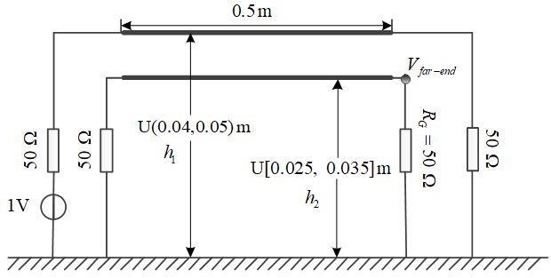
Fig. 6. The uncertainty analysis problem in the reference [8].
The heights of the two conductors are uncertain, and the height of the radiating conductor obeys uniform distributionwhile the height of the disturbed conductor obeys uniform distribution . Using a random variable model to describe this uncertainty factor, the following relationship can be obtained:
| (9) |
| (10) |
where and both stand for the uniform distribution .
For the SROM, the random variables and are sampled first, and a fixed number of feature points are selected. Then, single deterministic EMC simulation is performed on each feature point, and the final uncertainty simulation result can be obtained. More details about the SROM can be found in reference [9]. The uncertainty analysis is realized respectively when the number of feature points is 2, 4, 8, and 16. The number of feature points represents the number of deterministic simulations required. Therefore, the smaller the number of feature points, the shorter the simulation time. Using the improved MEAM, Table 2 shows the convergence determination process of the SROM.
Table 2: Convergence determination process of the SROM
| Number of Feature Points | The Common Area Value |
| 2 times and 4 times | 0.5337 |
| 4 times and 8 times | 0.7235 |
| 8 times and 16 times | 0.9606 |
According to Table 2, the number of convergence feature points of SROM in this example is 16. It is worth noting that only two feature points will not be used in actual simulation process. In this article, this selection is to better show the convergence process of the SROM.
In uncertainty analysis field, the results of the MCM are usually regarded as the standard answer. This paper also compares the SROM results under different times with the MCM results, as shown in Figure 7 and Figure 8. Figure 7 presents the expectation results, and Figure 8 gives the standard deviation results.
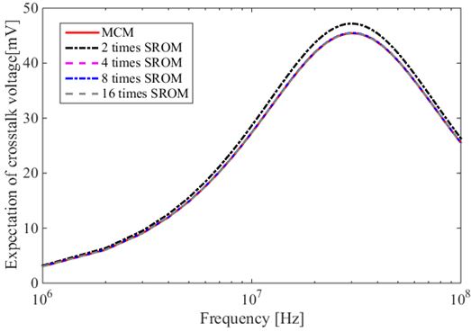
Fig. 7. Expectation results of the SROM.
In Figure 7, except two times SROM, the other results are close to the MCM results. It shows that when the number of feature points is 4, the estimate of expectation is accurate. In contrast to Figure 8, the SROM result is accurate only when the number of feature points is greater than 8. Obviously, when the feature point is 8, the algorithm is close to convergence. However, in order to ensure that the SROM completely converges, it is considered that 16 is the number of true convergent feature points.
In order to further describe the convergence process, the FSV method is introduced to quantify the difference between the MCM results and the SROM results in Figure 7 and Figure 8, as shown in Table 3. More details about the FSV method can be obtained in the references [11] and [12].
According to the FSV results in Table 3, it is clearly shown that 16 is the number of convergent feature points.

Fig. 8. Standard deviation results of the SROM.
Table 3: FSV results of the SROM under different times
| Expectation | Standard Deviation | |
| MCM and 2 times SROM | 0.0492 | 0.7615 |
| MCM and 4 times SROM | 0.0003 | 0.4763 |
| MCM and 8 times SROM | 0.0017 | 0.0205 |
| MCM and 16 times SROM | 0.0005 | 0.0144 |
In this example, the simulation time of the MCM is 642.57 s, while that of the SROM is only 1.68 s. It proves the unique advantage of the SROM in computational efficiency.
In summary, the improved MEAM can accurately determine the convergence of the SROM.
V. DISCUSSION
A. Convergence decision of the MCM
The number of basic sampling points N is determined first, and usually N is several hundred times. Then, the uncertainty analysis is respectively performed by using the MCM when the number of sampling points is N and . Based on the improved MEAM, the common area value between the uncertainty analysis results is calculated. If the area value is greater than 0.95, is the number of convergent sampling points. Otherwise, MCM must be used for simulation under the sampling points , and so on, until the common area value between the uncertainty analysis results of adjacent sampling points is greater than 0.95.
In the calculation example of Section IV, N is selected as 800, and the algorithm has converged when the number of sampling points is 6400.
B. Convergence decision of the SGM and the SCM
Whether it is the SGM or the SCM, the uncertainty analysis results are calculated first when the chaotic polynomial orders are 2 and 3. The improved MEAM is applied to calculate the common area value between adjacent order results. If the area value is greater than 0.95, the convergence order is 3. Otherwise, the uncertainty analysis result must continue to calculate with chaotic polynomial order 4, 5, and so on, until the common area value between adjacent order results is greater than 0.95.
VI. CONCLUSION
In this paper, the improved MEAM is proposed to solve the problem of convergence determination of uncertainty analysis methods in the EMC simulation field. It is certified that the proposed method not only retains the advantages of the conventional MEAM in standardization and generalization, but also calculates the common area values more accurately. Using a calculation example in published reference, the improved MEAM successfully achieves the convergence determination of the SROM. Finally, the promotion of the improved MEAM in convergence determination for three famous uncertainty analysis methods (MCM, SGM, and SCM) is also described.
REFERENCES
[1] C. F. M. Carobbi, S. Lalléchère, and L. R. Arnaut, “Review of uncertainty quantification of measurement and computational modeling in EMC part I: measurement uncertainty,” IEEE Transactions on Electromagnetic Compatibility, vol. 61, no. 6, pp. 1690-1698, Dec. 2019.
[2] A. Kriz, “Uncertainty calculation for AMN impedance contribution using the Monte Carlo Method,” 2019 IEEE International Symposium on Electromagnetic Compatibility, Signal & Power Integrity, pp. 565-569, Jul. 2019.
[3] E. Amador, C. Lemoine, and P. Besnier, “Optimization of immunity testing in a mode tuned reverberation chamber with Monte Carlo simulations,” 2012 ESA Workshop on Aerospace EMC, Venice, pp. 1-6, Jul. 2012.
[4] S. K. Goudos, E. E. Vafiadis, and J. N. Sahalos, “Monte Carlo simulation for the prediction of the emission level from multiple sources inside shielded enclosures,” IEEE Transactions on Electromagnetic Compatibility, vol. 44, no. 2, pp. 291-308, May 2002.
[5] P. Manfredi, D. Vande Ginste, D. De Zutter, and F. G. Canavero, “Generalized decoupled polynomial chaos for nonlinear circuits with many random parameters,” IEEE Microwave and Wireless Components Letters, vol. 25, no. 8, pp. 505-507, Aug. 2015.
[6] P. Manfredi and F. G. Canavero, “Numerical calculation of polynomial chaos coefficients for stochastic per-unit-length parameters of circular conductors,” IEEE Transactions on Magnetics, vol. 50, no. 3, pp. 74-82, Mar. 2014.
[7] X. Wu, F. Grassi, P. Manfredi, and D. Vande Ginste, “Efficiency of the perturbative stochastic Galerkin method for multiple differential PCB lines,” 2018 IEEE Electrical Design of Advanced Packaging and Systems Symposium, pp. 1-3, Dec. 2018.
[8] J. Bai, G. Zhang, D. Wang, A. P. Duffy, and L. Wang, “Performance comparison of the SGM and the SCM in EMC simulation,” IEEE Transactions on Electromagnetic Compatibility, vol. 58, no. 6, pp. 1739-1746, Dec. 2016.
[9] Z. Fei, Y. Huang, J. Zhou, and Q. Xu, “Uncertainty quantification of crosstalk using stochastic reduced order models,” IEEE Transactions on Electromagnetic Compatibility, vol. 59, no. 1, pp. 228-239, Feb. 2017.
[10] J. Bai, L. Wang, D. Wang, A. P. Duffy, and G. Zhang, “Validity evaluation of the uncertain EMC simulation results,” IEEE Transactions on Electromagnetic Compatibility, vol. 59, no. 3, pp. 797-804, Jun. 2017.
[11] A. P. Duffy, A. Orlandi, and G. Zhang, “Notice of retraction: review of the feature selective validation method (FSV). Part I—Theory,” IEEE Transactions on Electromagnetic Compatibility, vol. 60, no. 4, pp. 814-821, Aug. 2018.
[12] A. Orlandi, A. P. Duffy, and G. Zhang, “Notice of retraction: review of the feature selective validation method (FSV). Part II - Performance analysis and research fronts,” IEEE Transactions on Electromagnetic Compatibility, vol. 60, no. 4, pp. 1029-1035, Aug. 2018.
BIOGRAPHIES

Jinjun Bai received the B.Eng. degree in electrical engineering and automation in 2013, and Ph.D. degree in electrical engineering in 2019 from the Harbin Institute of Technology, Harbin, China. At present, Mr. Bai is a lecturer at Dalian Maritime University. His research interests include uncertainty analysis methods in EMC simulation, EMC problem of electric vehicles, and the validation of CEM.

Jingchao Sun received the B.Eng. and M.Eng. degrees in electrical engineering from Dalian Maritime University, Dalian, China, in 2009 and 2012, respectively, where she is currently pursuing the Ph.D. degree. She is currently an Electrical Engineer with the Dalian Electric Traction Research and Development Center, China CNR Corporation Ltd., Dalian. Her current research interests include unmanned crafts and their intelligent modeling and control.

Ning Wang received his B.Eng. degree in Marine Engineering and the Ph.D. degree in control theory and engineering from the Dalian Maritime University, Dalian, China in 2004 and 2009, respectively. From September 2008 to September 2009, he was financially supported by China Scholarship Council to work as a joint-training PhD student at the Nanyang Technological University (NTU), Singapore. In view of his significant research at NTU, he received the Excellent Government-funded Scholars and Students Award in 2009. From August 2014 to August 2015, he worked as a Visiting Scholar at the University of Texas at San Antonio. His research interests include self-learning modeling and control, unmanned (marine) vehicles, machine learning, and autonomous systems. Dr. Wang received the Nomination Award of Liaoning Province Excellent Doctoral Dissertation, and also won the State Oceanic Administration Outstanding Young Scientists in Marine Science and Technology, the China Ocean Engineering Science and Technology Award (First Prize), the Liaoning Province Award for Technological Invention (First Prize), the Liaoning Province Award for Natural Science (Second Prize), the Liaoning Youth Science and Technology Award (Top10 Talents), the Liaoning BaiQianWan Talents (First Level), the Liaoning Excellent Talents (First Level), the Science and Technology Talents the Ministry of Transport of the P. R. China, the Youth Science and Technology Award of China Institute of Navigation, and the Dalian Leading Talents. He has authored three books, and more than 100 SCI-indexed journal papers. He currently serves as a member of IEEE TC on Industrial Informatics, the American Society of Mechanical Engineers (ASME), the Society of Naval Architects and Marine Engineers (SNAME), the Chinese Association of Automation (CAA), and the China’s Society of Naval Architecture and Marine Engineering (CSNAME). He has been Leading Guest Editors of the International Journal of Fuzzy Systems, the International Journal of Advanced Robotics System, the Advances in Mechanical Engineering, and the International Journal of Vehicle Design. He currently serves as Editorial Board Members and Associate Editors of the International Journal of Fuzzy Systems, the Electronics (MDPI), the Journal of Electrical Engineering & Technology, the Cyber-Physical Systems (Taylor-Francis), the Frontiers in Robotics and AI, and the International Journal of Aerospace System Science and Engineering.
ACES JOURNAL, Vol. 36, No. 11, 1446–1452.
doi: 10.13052/2021.ACES.J.361108
© 2021 River Publishers