Convergence Acceleration of Infinite Series Involving the Product of Riccati–Bessel Function and Its Application for the Electromagnetic Field: Using the Continued Fraction Expansion Method
Zheng Fanghua, Di Qingyun, Yun Zhe, and Gao Ya
1CAS Engineering Laboratory for Deep Resources Equipment and Technology, Institute of Geology and Geophysic, Chinese Academy of Sciences, Beijing 100029, China
2Innovation Academy for Earth Science, Chinese Academy of Sciences, Beijing 100029, China
3University of Chinese Academy of Sciences, Beijing 100049, China
Zhengfanghua18@mails.ucas.ac.cn; qydi@mail.iggcas.ac.cn; yz791161833@163.com; gaoya171@mails.ucas.ac.cn
Submitted On: September 2, 2021; Accepted On: November 4, 2021
Abstract
A summation technique has been developed based on the continuous fractional expansion to accelerate the convergence of infinite series involving the product of Riccati–Bessel functions, which are common to electromagnetic applications. The series is transformed into a new and faster convergent sequence with a continued fraction form, and then the continued fraction approximation is used to accelerate the calculation. The well-known addition theorem formula for spherical wave function is used to verify the correctness of the algorithm. Then, some fundamental aspects of the practical application of continuous fractional expansion for Mie scattering theory and electromagnetic exploration are considered. The results of different models show that this new technique can be applied reliably, especially in the electromagnetic field excited by the vertical electric dipole (VED) source in the “earth-ionospheric” cavity. The comparison among the new technology, the Watson-transform, and the spherical harmonic series summation algorithm shows that this new technology only needs less than 120 series items which is already enough to obtain a small relative error, which greatly improves the convergence speed, and provides a new way to solve the problem.
Index Terms: infinite series; Riccati–Bessel function; Mie scattering; electromagnetic prospecting.
I. INTRODUCTION
The study of electromagnetism can be applied in many areas, such as electromagnetic scattering [1, 2, 3, 4, 5], plasmonics [6, 7, 8], seismo-ionospheric disturbance [9, 10, 11], radio communication [12, 13, 14, 15], and earth science [16, 17, 18, 19, 20] studies. Following the pioneering work of Lorenz-Mie [21], the subject of electromagnetic wave propagation under spherical boundary has become a hot spot in the fields of electromagnetism [1, 2, 3, 4, 5, 14, 15, 16, 22]. Since the spherical Bessel function is often used as the eigenfunction for the spherical coordinate system, the numerical calculation including the integral or series of the spherical Bessel function is extremely important in the fields of scientific calculation and engineering applications [23, 24]. Theoretically, the analytical solution of the Helmholtz equation in the spherical coordinate system can be obtained by the method of separating variables. However, even if modern high-performance computers are used to calculate the sum of the series directly item by item, the spherical Bessel function of high-order complex parameters can easily lead to a numerical overflow in the calculation process [25, 26]. As a result, the series expression does not converge, and it is time-consuming to directly calculate the infinite sum.
To overcome this computational burden, predecessors proposed different solutions to specific series problems [27, 28, 29]. For the Mie scattering series, for example, Wiscombe [30] proposed to truncate the series and give the maximum summation term Nmax. The Wiscombe criterion is by far the most widely used, but the criterion is based on a priori estimation [31], and Nmax is positively correlated with the frequency and the radius of the sphere. That is, the truncation terms will increase with the increase in frequency and radius. In addition, the truncation formula cannot be fully applied to the spherical vector wave function. For earth-scale models, it is time-consuming to directly calculate the infinite sum. Fock [32] put forward the Watson-transform technique to transform the infinite series summation into a contour integral and obtained the expression that is convenient for engineering calculations. But the realization of the Watson-transform depends on the solution of the poles of the summation function in the series, which is complicated. Wang [22] developed the spherical harmonic series acceleration convergence algorithm proposed by Barrick, but it needs to subtract an appropriate closed-form expression from the original accurate series, and then add the same closed-form expression to improve the convergence.
The principle of the infinite series acceleration method is to transform a slowly convergent sequence into a new, faster converging sequence. Since there is not any general algorithm that could work well for every type of sequence, we should try different algorithms to obtain the optimum result for the problem under investigation [28]. Continued fraction expansion has wide application in the numerical calculation of special analytic functions. Hänggi [27] applied the method of the continued fraction expansion for the slow convergent series which occurs in quantum mechanics and statistical mechanics. In this paper, the author tries to apply the continued fraction expansion to improve the convergence of infinite series containing the product of spherical Bessel functions, aiming to find a simpler and more efficient method to converge the series. The comparison with previous results shows that this new technology can be reliably applied, especially for the calculation of the field excited by the electric dipole source in the “earth-ionospheric” cavity, and provides a new way to solve the problems.
II. BASIC PROPERTIES OF THE CONTINUED FRACTIONS
A. Continued fraction expansion of the series
If the infinite series satisfies the form:
| (1) |
Expand the series (1) into continued fraction form at y =1, we have:
| (2) |
where is the nth continued fraction factor [27], n is the total number of factors, and eqn (2) is named the limit periodic continued fraction. Define a global array with an initial value of “0,” intermediate variables and , then the relationship between the continued fraction factor and the series is [27]:
when ,
| (3) |
where and are loop variables, is a rounding function, and means interchange and .
B. Convergence algorithm for continued fractions
Starting from the right side of eqn (2), one can gradually approach the convergence value of the series , but each additional term in the calculation means recalculating the entire continued fraction. Therefore, Wallis [33] proposed a fast recursive algorithm, define the array and with an initial value: , , , . And the relationship between , and is:
| (4) |
And we have:
| (5) |
From eqn (2), (4), and (5), the successive approximation to infinite continued fraction can be calculated until the required accuracy is obtained. But the recursive algorithm is easy to cause calculation overflow because the values of and are too large or too small. Define , , we have [34]:
| (6) |
| (7) |
| (8) |
Define , , , from eqn (5) and (8) we have:
| (9) |
Eqn (9) describes the nth approximate value represented by the continued fraction, where the value of n depends on the oscillation of the Bessel function and the required accuracy. Therefore, it is necessary to specify a small positive number according to the required calculation accuracy. When the relative error of the last two calculation results is less than or equal to , that is, when the eqn (10) is established, the series is considered to be convergent, and .
| (10) |
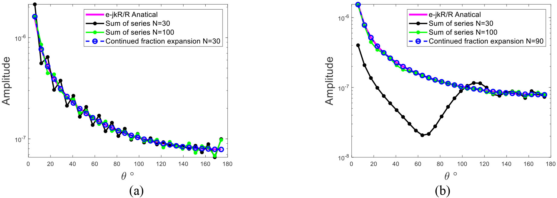
Figure 1: Comparison of the free-space spherical wave function obtained by the continued fraction expansion method and the direct summation. N is the number of items, and the relative accuracy is 10. (a) f = 1Hz, (b) f = 300Hz.
III. EXAMPLES
To investigate the approximation effect of the continued fraction expansion of infinite series containing Bessel function, we choose the addition theorem formula [15] of the spherical wave function in free space to verify the correctness of the algorithm:
| (11) |
where and are the spherical Bessel functions, is the wavenumber of free space, is the radius of the earth, is the position of the field source, is the distance from the observation point to the source.
Figure 1 shows the calculation results of direct series summation and continued fraction expansion summation. The frequency , , , . To further show the numerical characteristics of the technique in this paper, in Figure 2, we show the number of items in the continued fraction expansion required at different frequencies and different observation positions and the number of terms required for the direct summation of the series.
It can be seen from Figure 1 and Figure 2 that the result of the continued fraction expansion is completely consistent with the analytical solution. As the frequency increases, the oscillation of the spherical Bessel function increases. It is necessary to increase the calculation items to obtain higher accuracy. It is worth noting that even at 300 Hz, the continued fraction expansion method only needs no more than 100 items, the effect and speed are much better than the direct summation method. At the same frequency, the farther away from the field source, the faster the series converges, and the closer to the field source, the slower the convergence speed. That is, we need to accurately calculate the high-order spherical Bessel function.
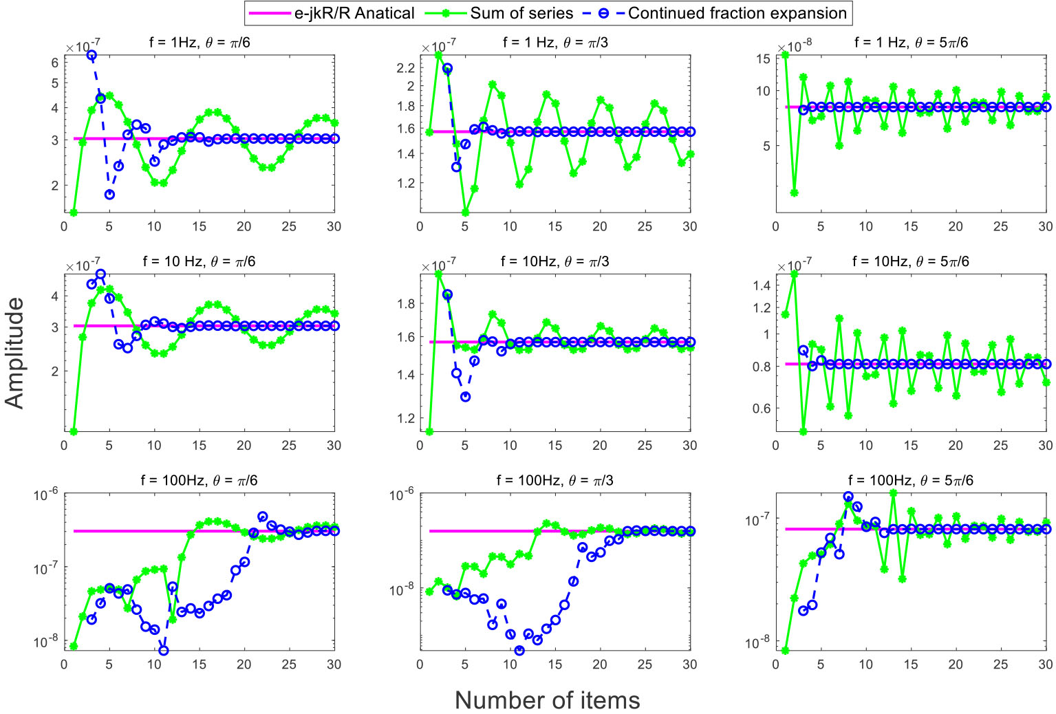
Figure 2: Comparison of the number of items required forthe continued fraction expansion and the direct summation.
IV. APPLICATION OF CONTINUED FRACTION EXPANSIONS FOR ELECTROMAGNETIC FIELD
A. Expressions for Mie series
The Lorenz–Mie theory [21] is a complete theoretical framework for studying the electromagnetic scattering of plane waves by a uniform isotropic media sphere. Consider a uniform sphere of radius a and embedded in a non-absorbing medium with a dielectric constant of M. For an incident monochromatic plane wave of wavelength , the electromagnetic characteristics of the incident beam can be described by a set of dimensionless scattering coefficients Q, extinction coefficients Q, absorption coefficients Q, and backscattering coefficients Q [5]:
| (12) |
where a and b are the Mie coefficients that characterize the optical response of the sphere:
where is the particle size parameter, is the relative refractive index, and are the Riccati–Bessel functions.
Figure 3 shows the calculation results of metal materials (m = 50+50i) in the range of particle size parameter x from 0 to 30 and compares them with the calculation results of Christian Mätzler [5]. It can be seen from Figure 3 that the two algorithms are in good agreement. The parameter with the maximum value and the maximum fluctuation is Q. The curves of Q and Q are closely connected near the value 2 and increase rapidly. For x = 30, N= 44, and N= 58. For the Mie series, the convergence of the original series is good enough, so the application of the continued fraction method does not bring a significant improvement in convergence, but it proves the correctness and practicability of our method. Note that as the particle size parameter x increases, the number of truncation items required for the series will increase. In Mätzler [5], for large parameters, the high-order spherical Bessel function leads to the overflow. The accurate calculation of high-order spherical Bessel functions can be found in theliterature [25], [26].
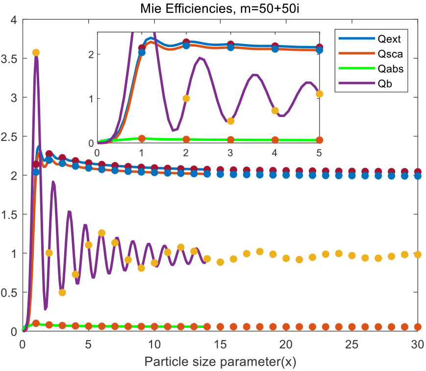
Figure 3: Mie Efficiencies for a metal-like material (m=50+50i) over the x range from 0 to 30. The solid lines are computed with the Wiscombe criterion, the dotted lines are calculated using the continued fraction expansion.
B. Propagation of ELF/SLF electromagnetic waves
In recent years, the propagation of ELF/SLF electromagnetic waves in the “earth-ionospheric” cavity has attracted much attention in the fields of submarine communication, resource exploration, earthquake precursor monitoring, and space weather disaster investigation [14, 15, 19, 22, 35].
Considering the vertical electric dipole source (VED) located near the spherical surface, the electromagnetic field on the earth’s surface can be represented as [14]:
| (13) |
where b and c are coefficients related to the electrical characteristics of the ionosphere and the earth, and and are the Riccati–Bessel function.
Different from the Mie scattering series, which only contains the product of the spherical Bessel function once, the ELF/SLF electromagnetic field excited by an electric dipole contains the product of the spherical Bessel function multiple times and the product of the Legendre function. Due to the scale of the earth, it is difficult to obtain accurate spherical Bessel function values of high-order complex parameter unless it is properly approximated [36]. Therefore, even with a high-performance computer, it is hard to converge the series by calculating the sum of the sequence item by item. Wait [15] adopted the classical modal theory and applied the Watson-transform to solve the radial electric field excited by a VED. Barrick [36] derived the spherical harmonic series expression of ELF/SLF electromagnetic wave field under ideal boundary conditions. Wang [22] developed Barrick’s method and proposed a numerical convergence algorithm, but it needs to subtract a closed-form expression from the original exact series, and then add the same closed expression to modify thesummation.
To verify the correctness and practicability of the new sequence, Figure 4 compares the radial electric field strength at 5 and 50 Hz with the asymptotic solution of Wait [15] and the numerical sum of Barrick [36]. At 50 Hz, the approximate solution obtained by Wait [15] using the classic Watson transform works well far away from the source, but it fails to show the rapid attenuation trend of the field in the region closer to the source. That is, near the source point, the electromagnetic field has the largest value and then decays rapidly, and finally shows the well-known resonance phenomenon. At 5 Hz, the difference of approximate solution increases significantly. Since both the paper and Barrick’s research adopt precise series solutions, the two curves are in good agreement, and the electromagnetic field near the source shows a clear downward trend. However, Barrick achieved sufficient accuracy and convergence by taking 650 items in the sequence, while it only needs no more than 120 items to obtain a relative accuracy of 10 by the algorithm in this paper, of which no more than 50 items in the far-field. Therefore, the algorithm in this paper can greatly improve the convergence speed. Therefore, only a few items are already enough to obtain a small relative error, which greatly improves the convergence speed.
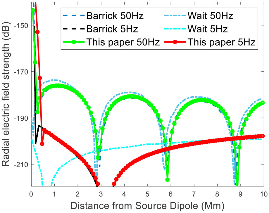
Figure 4: Compare the radial electric field strength at 5 and 50 Hz with the asymptotic solution of Wait [15] and the numerical sum of Barrick [36].
C. Application in electromagnetic prospecting
As one of the important methods of resource and energy exploration, electromagnetic exploration is based on the difference in resistivity and polarizability between the ore body and the surrounding rock. Different from signal transmission in the communication field, geophysical prospecting needs to construct the electrical parameters of underground media from the information carried by electromagnetic waves.
As a new electromagnetic exploration method, the wireless electromagnetic method (WEM) has the advantages of high signal strength, good consistency, wide application range, large exploration depth, etc., and has a broad application prospect in deep resource exploration [19]. By measuring the spatial distribution of electromagnetic fields caused by different rocks and ores, the electrical parameters of underground media can be constructed, thus to detect underground targets. Following the expression (13), define the ratio of the orthogonal electric field to the magnetic field on the earth’s surface as the spherical wave impedance [15]:, in the extremely low-frequency range: [35]. Although it is not possible to define an idealized plane wave source on the spherical earth model, fortunately, Di [19] pointed out that when the transmission distance is greater than six skin depths, the ELF/SLF electromagnetic wave field can be regarded as a plane wave source. And the apparent resistivity and phase in the spherical coordinate are:
| (14) |
To verify the feasibility of WEM in the spherical earth and analyze its response characteristics, Figure 5 shows the apparent resistivity and phase of the WEM in the homogeneous earth model with earth resistivity of , 100 and 1000.
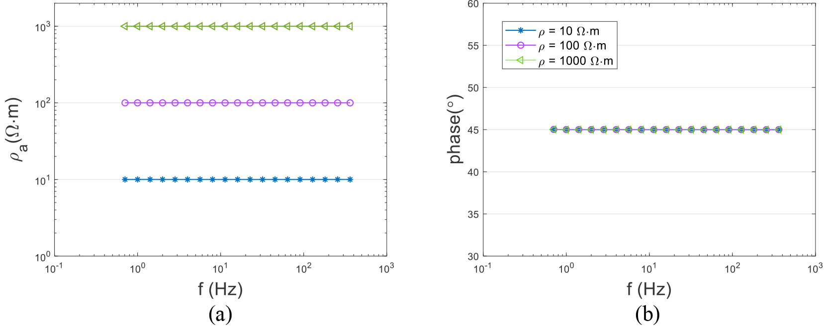
Figure 5: WEM apparent resistivity (a) and phase (b) calculated for the homogeneous models. The transmit frequency is 2 Hz, n = -0.5:0.5:8.5, and the interval is 0.5, and the observation azimuth is 10 degrees.
Figure 5(a) shows that in the ELF/SLF range, the apparent resistivity curve of WEM at different frequencies is completely coincident with the resistivity of the earth. Because in eqn (14), it can be seen that the ratio of the electric field and the magnetic field is closely related to the emission frequency and the resistivity of the underground medium. Therefore, when the emission frequency is known, the resistivity of the underground medium can be obtained, which reveals that WEM can detect the electrical parameters of underground targets. In addition, following the definition of skin depth , it can be known that in the earth media, the attenuation rate of electromagnetic waves is proportional to the square root of its working frequency. Therefore, WEM has obvious advantages in deep resource exploration due to its lower operating frequency. Figure 5 (b) shows that for a homogeneous earth model, the phase is /4, which is independent of the frequency and the electrical parameters of the underground media. This is consistent with the conclusion that the phase of the magnetic field in a homogeneous medium lags the phase of the electric field by /4, and further proves the correctness of WEM.
V. CONCLUSION
In this paper, a summation technique based on Continued fraction is developed to accelerate the convergence of infinite series containing the product of Riccati–Bessel functions, which are common in electromagnetic problems. And the recursive algorithm needed for effective calculation of Continued fraction coefficients is presented, so that the series is transformed into a new and faster convergent sequence in the form of continued fractions, then the Continued fraction approximation is used to accelerate the calculation. In addition, some main aspects of the practical application of continuous fractional expansion in Mie scattering theory and electromagnetic exploration are considered. The results show that in the Mie scattering model, since the convergence of the original series is good enough, the application of the Continued fraction expansion does not bring significant improvement. However, the new technology has powerful advantages for the calculation of extremely low-frequency electromagnetic fields. It only needs no more than 120 series items to obtain a relative accuracy of 10, of which no more than 50 items in the far-field. Therefore, only a few operations can be performed to obtain a small relative error, which greatly improves the convergence speed.
ACKNOWLEDGEMENTS
This work was supported part by the Scientific Instrument Developing Project of the Chinese Academy of Sciences under Grant ZDZBGCH2018006, and in part by the National Natural Science Foundation of China under grant number 41874088.
REFERENCES
[1] G. Ruello and R. Lattanzi, “Scattering from spheres: A new look into an old problem,” Electronics, vol. 10, no. 2, pp. 216, 2021.
[2] W. Zhuang, R. Li, J. Liang, and Y. Jia, “Debye series expansion for light scattering by a charged sphere,” Applied Optics, vol. 60, no. 7, pp. 1903-1915, 2021.
[3] C. Gao, B. Sun, and Y. Zhang, “Electromagnetic wave scattering by charged coated spheres,” Journal of Quantitative Spectroscopy and Radiative Transfer, vol. 272, pp. 107757, 2021.
[4] S. Batool, F. Frezza, F. Mangini, and X. Yu-Lin, “Scattering from multiple PEC sphere using translation addition theorems for spherical vector wave function,” Journal of Quantitative Spectroscopy and Radiative Transfer, vol. 248, pp. 106905, 2020.
[5] C. Mätzler, MATLAB Functions for Mie Scattering and Absorption, Version 2, 2002.
[6] M. E. Nazari and W. Huang, “Asymptotic solution for the electromagnetic scattering of a vertical dipole over plasmonic and non-plasmonic half-spaces,” IET Microwaves, Antennas & Propagation, vol. 15, pp. 704-717, 2021.
[7] B. Beiranvand, A. S. Sobolev, and A. Sheikhaleh, “A proposal for a dual-band tunable plasmonic absorber using concentric-rings resonators and mono-layer graphene,” Optik, vol. 223, pp. 165587, 2020.
[8] M. Gingins, M. Cuevas, and R. Depine, “Surface plasmon dispersion engineering for optimizing scattering, emission, and radiation properties on a graphene spherical device,” Applied Optics, vol. 59, no. 14, pp. 4254-4262, 2020.
[9] S. Zhao, X. Shen, C. Zhou, L. Liao, Z. Zhima, and F. Wang, “The influence of the ionospheric disturbance on the ground based VLF transmitter signal recorded by LEO satellite–Insight from full wave simulation,” Results in Physics, vol. 19, pp. 103391, 2020.
[10] M. Hayakawa, A. P. Nickolaenko, Y. P. Galuk, and I. G. Kudintseva, “Scattering of extremely low frequency electromagnetic waves by a localized seismogenic ionospheric perturbation: observation and interpretation,” Radio Science, vol. 55, no. 12, pp. 1-26, 2020.
[11] R. Song, K. Hattori, X. Zhang, and S. Sanaka, “Seismic-ionospheric effects prior to four earthquakes in Indonesia detected by the China seismo-electromagnetic satellite,” Journal of Atmospheric and Solar-Terrestrial Physics, vol. 205, pp. 105291, 2020.
[12] S. Chowdhury, S. Kundu, T. Basak, S. Ghosh, M. Hayakawa, S. Chakraborty, and S. Sasmal, “Numerical simulation of lower ionospheric reflection parameters by using international reference ionosphere (IRI) model and validation with very low frequency (VLF) radio signal characteristics,” Advances in Space Research, vol. 67, no. 5, pp. 1599-1611, 2021.
[13] C. Dong, Y. He, M. Li, C. Tu, Z. Chu, X. Liang, and N. X. Sun, “A portable very low frequency (VLF) communication system based on acoustically actuated magnetoelectric antennas,” IEEE Antennas and Wireless Propagation Letters, vol. 19, no. 3, pp. 398-402, 2020.
[14] W. Pan and K. Li, Propagation of SLF/ELF Electromagnetic Waves. Springer Science & Business Media, 2014.
[15] J. R. Wait, Electromagnetic Waves in Stratified Media: Revised Edition Including Supplemented Material. Elsevier, 2013.
[16] Y. Gao, Q. Di, R. Wang, C. Fu, et al., “Strength of the electric dipole source field in multilayer spherical media,” IEEE Transactions on Geoscience and Remote Sensing, 2021.
[17] Q. Di, C. Fu, Z. An, et al., “An application of CSAMT for detecting weak geological structures near the deeply buried long tunnel of the Shijiazhuang-Taiyuan passenger railway line in the Taihang Mountains,” Engineering Geology, vol. 268, pp. 105517, 2020.
[18] Q. Di, G. Xue, C. Fu, and R. Wang, “An alternative tool to controlled-source audio-frequency magnetotellurics method for prospecting deeply buried ore deposits,” Science Bulletin, vol. 65, no. 8, pp. 611-615, 2020.
[19] Q. Di, M. Wang, C. Fu, et al., Study on the Characteristics of Electromagnetic Wave Propagation in Earth-Ionosphere Mode, Science Press, 2013.
[20] D. Shreeja, et al. “Application of Fracture Induced Electromagnetic Radiation (FEMR) technique to detect landslide-prone slip planes,” Natural Hazards, vol. 101, no. 2, 2020.
[21] G. Mie, “Articles on the optical characteristics of turbid tubes, especially colloidal metal solutions,” Ann. Phys, vol. 330, pp. 377-445, 1908.
[22] Y. X. Wang, R. H. Jin, J. P. Geng, et al., “Exact SLF/ELF underground HED field strengths in earth-ionosphere cavity and Schumann resonance,” IEEE Transactions on Antennas and Propagation, vol. 59, no. 8, pp. 3031-3039, 2011.
[23] M. Tezer, “On the numerical evaluation of an oscillating infinite series,” Journal of Computational and Applied Mathematics, vol. 28, pp. 383-390, 1989.
[24] M. Toyoda and T. Ozaki, “Fast spherical Bessel transform via fast Fourier transform and recurrence formula,” Computer Physics Communications, vol. 181, no. 2, pp. 277-282, 2010.
[25] W. J. Lentz, “Generating Bessel functions in Mie scattering calculations using continued fractions,” Applied Optics, vol. 15, no. 3, pp. 668-671, 1976.
[26] D. M. O’Brien, “Spherical Bessel functions of large order,” Journal of Computational Physics, vol. 36, no. 1, pp. 128-132, 1980.
[27] P. Hänggi, F. Rösel, and D. Trautmann, “Continued fraction expansions in scattering theory and statistical non-equilibrium mechanics,” Zeitschrift Für Naturforschung A, vol. 33, no. 4, pp. 402-417, 1978.
[28] N. Kinayman and M. I. Aksun, “Comparative study of acceleration techniques for integrals and series in electromagnetic problems,” Radio Science, vol. 30, no. 6, pp. 1713-1722, 1995.
[29] F. G. Mitri, “Partial-wave series expansions in spherical coordinates for the acoustic field of vortex beams generated from a finite circular aperture,” IEEE Transactions on Ultrasonics, Ferroelectrics, and Frequency Control, vol. 61, no. 12, pp. 2089-2097, 2014.
[30] W. J. Wiscombe, “Improved Mie scattering algorithms,” Applied Optics, vol. 19, no. 9, pp. 1505-1509, 1980.
[31] J. R. Allardice and R. E. C. Le, “Convergence of Mie theory series: criteria for far-field and near-field properties,” Applied Optics, vol. 53, no. 31, pp. 7224-7229, 2014.
[32] V. A. Fock, Electromagnetic Diffraction and Propagation Problems, Pergamon Press, 1965.
[33] W. H. Press, W. H. Press, B. P. Flannery, et al., Numerical Recipes in Pascal: The Art of Scientific Computing, Cambridge University Press, 1989.
[34] J. Wallis and W. Johannis, Opera Mathematica, vol. 3, 1972.
[35] Y. Yuan, Propagation and Noise of Ultra-Low Frequency and Extremely Low Frequency Electromagnetic Waves, National Defense Industry Press, 2011.
[36] D. E. Barrick, “Exact ULF/ELF dipole field strengths in the earth-ionosphere cavity over the Schumann resonance region: idealized boundaries,” Radio Science, vol. 34, no. 1, pp. 209-227, 1999.
BIOGRAPHIES
Fang-hua Zheng was born in Luzhou, Sichuan, China, in 1995. He received a bachelor’s degree in exploration technology and engineering from the Southwest Petroleum University in Chengdu, China, in 2018. He is currently pursuing the Ph.D. degree in geophysics at University of Chinese Academy of Sciences, Beijing, China. His current research interests include the propagation of SLF/ELF electromagnetic waves in the “earth-ionosphere” cavity and its applications in geophysical prospecting.
Qing-yun Di received the bachelor’s and master’s degrees from the Changchun College of Geology (now Jilin University), Jilin, China, in 1987 and 1990, respectively, and the Ph.D. degree from the Institute of Geology and Geophysics (IGG), Chinese Academy of Sciences (CAS), Beijing, China, in 1998. Dr. Di is a research fellow of geophysics at the CAS Engineering Laboratory for Deep Resources Equipment and Technology, IGGCAS. She has received a number of awards from the Chinese Government and CAS, including the National Science and Technology Progress Second Prize and the Outstanding Science and Technology Achievement Prize of CAS. She is researching the propagation characteristics of controlled-source EM waves, putting into consideration the ionosphere, atmosphere, and the earth. Her research activities are mainly devoted to research and development of EM method instruments, forward modeling, and inversion of controlled source audio-frequency magnetotellurics (CSAMT), electrical resistivity tomography (ERT), and ground-penetrating radar (GPR) methods.
Zhe Yun received the B.S. degree in Geo-exploration Technology and Engineering from the Ocean University of China, Qingdao, China, in 2020. He is currently pursuing the M.S. degree in geophysics at the Institute of Geology and Geophysics (subordinate to the Innovation Academy for Earth Science), and the College of Earth and Planetary Sciences, University of the Chinese Academy of Sciences. His research interests include the controlled source electromagnetic data forward modeling and inversion.
Ya Gao received the B.S. degree in Geophysics from the Jilin University, Jilin, China, in 2017. She is currently pursuing the Ph.D. degree at the Key Laboratory of Shale Gas and Engineering, Institute of Geology and Geophysics (subordinate to the Innovation Academy for Earth Science), and the College of Earth and Planetary Sciences, University of the Chinese Academy of Sciences. Her research interests cover the controlled source electromagnetic data forward modeling and inversion.
ACES JOURNAL, Vol. 36, No. 12, 1518–1525.
doi: 10.13052/2021.ACES.J.361202
© 2021 River Publishers