New Approximate Expressions for Evaluating the Fields of a Vertical Magnetic Dipole in a Dissipative Half Space

Hongyun Deng, Gaobiao Xiao, and Shifeng Huang

Key Laboratory of Ministry of Education of Design and Electromagnetic Compatibility of High Speed Electronic Systems, Shanghai Jiao Tong University, Shanghai 200240, China

hongyundeng@sjtu.edu.cn; gaobiaoxiao@sjtu.edu.cn; huangshifeng@sjtu.edu.cn

Submitted On: September 10, 2021; Accepted On: November 11, 2021

Abstract

In this paper, a set of new asymptotic approximate expressions for evaluating the electromagnetic (EM) fields generated by a vertical magnetic dipole placed in a dissipative half space is proposed. The lateral wave that guarantees the continuity of the EM fields at the interface is discussed in detail. Using the spectral method, the integral expressions of the field components are obtained. The dominant part is extracted from the lateral wave for large radial distance so that all field components in this situation can be approximately expressed with explicit expressions, which makes the method efficient. Besides, the proposed method has no restriction condition on the parameter choices of different half spaces, so it can be applied in more general situations. Some calculation results and comparisons are given to validate the effectiveness of this extraction method.

Index Terms: Asymptotic approximation, dissipative medium, lateral wave, spectral method, surface wave, magnetic dipole.

I. INTRODUCTION

The surface waves have been studied since the time of Sommerfeld [1]. In 1907, Zenneck discussed the waves crouching on the intersecting surface of the earth and the air that possesses the radial symmetry [2]. He wanted to explain the long-distance radio wave propagation on the earth by the surface wave over the ground. The discussion of the Zenneck wave is still going on, even if the long-distance propagation of the electromagnetic (EM) waves could be explained by the existence of the ionosphere nowadays. The study about such waves has its own meaning since it guarantees the continuity of the EM waves at the boundary of lossy media such as the earth, the sea water, and the sea crust [3, 4, 5, 6, 7, 8]. This kind of surface waves only exist when the source is placed near the boundary, which means that sources like plane waves cannot excite such kind of waves [9]. Norton simplified the Sommerfeld’s complicated integral solution of the surface waves by some approximations to give explicit expressions of the surface waves and make it more applicable [7]. On the other hand, Baños got further results following the work of Sommerfeld, but those were still too complicated [10]. They could not give the direct physical insight of the surface waves and were not convenient for engineering applications [3]. The surface waves excited by dipoles (electric and magnetic) placed near the boundary of dissipative medium are also called the lateral waves. It has many realistic application scenes such as communication with submerged submarines. King [3] gave an extensive discussion of the theory and application of the lateral waves generated by a vertical electric dipole in the sea. However, King’s asymptotic approximation method has the restriction condition on the wave numbers of the two half spaces that $\left|k_1\right|\gg \left|k_0\right|$, and this condition is satisfied by the relevant parameters of the sea and the air. Researchers also tried to get numerical solutions of the lateral waves that travel along the interface of the sea and the air with the help of computers. However, the numerical methods are time-consuming when calculating the far fields because the integrands of the integral expressions of the fields oscillate severely, and it needs some special techniques [11, 12, 13]. Nowadays, there are different methods that could deal with the EM field problem in planar stratified media [14, 15, 16, 17]. None of these methods could avoid the evaluation of Sommerfeld integrals and the evaluation of Sommerfeld integrals can be categorized into three types: the direct numerical method [18, 19, 20], the discrete complex image method [21, 22, 23], and the asymptotic method [3, 10]. The asymptotic method has the advantage of having high efficiency and being accurate when calculating the EM field in the far region.

In this paper, a novel asymptotic method to extract the dominant parts of the lateral waves is proposed. This method stems from the double saddle point method [10]. Nevertheless, no asymptotic series coefficients need to be specifically calculated like that in [10] due to the proposed extraction technique. All the field components generated by a vertical magnetic dipole (VMD; it can be regarded as a model of the closed electrical line carrying a time-varying electric current loop which supplies the electricity to the electronic devices on a ship) in a dissipative half space have explicit expressions by neglecting the corresponding residual integrals. The fields of other types of dipoles can be dealt with in a similar way. The newly proposed method has no restriction condition on the wavenumbers of different half spaces; so it can be applied in more general problems than King’s approximation method.

II. FORMULATION

A. Model

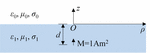
The basic model in this paper is depicted in Figure 1. Hereinafter, the cylindrical coordinate system is used, and the three coordinates are $(\rho ,\varphi ,z)$. Due to the radial symmetry, $\varphi$ is always assumed to be 0. The lower half space is sea, and the upper half space is air. The plane $z=0$ is the interface of the two half spaces. A VMD is placed in the sea at the point $(\rho ,z)=(0,-d)$ ($d>0$). M is the dipole moment. Assume that the permittivity and the permeability of the free space are ${ϵ}_0$ and ${\mu }_0$, respectively. The sea has the permittivity of ${ϵ}_1={81}_0$, the permeability of ${\mu }_1={\mu }_0$, and the conductivity of ${\sigma }_1=4$ S/m. The air has the permittivity of ${ϵ}_{\mathrm{0}}$, the permeability of ${\mu }_0$, and the conductivity of ${\sigma }_0=0$ S/m.

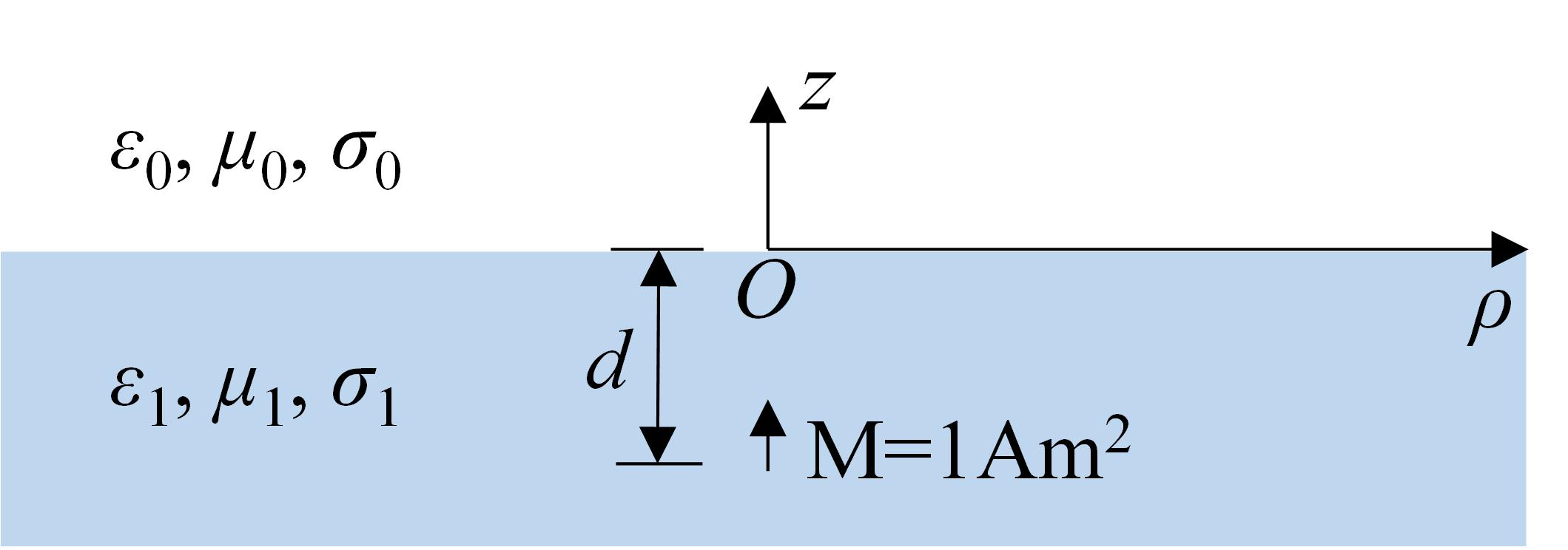
Fig. 1. A vertical magnetic dipole in the sea.

B. Integral expressions of the EM fields

Using the spectral method [24], the nonzero field components in the sea can be expressed as the following three integrals:

$$\begin{array}{c}{H}_{1z}={\int }_{-\mathrm{\infty }}^{\mathrm{\infty }}\mathit{d}{k}_{\rho }\left[\begin{array}{c}{e}^{i{k}_{1z}\left(z+d\right)}+\hfill \\ R{e}^{-i{k}_{1z}\left(z+d\right)}\hfill \end{array}\right]H_{\mathrm{VMD}}{H}_0^{\left(1\right)}\left(k_{\rho }\rho \right),\hfill \\ H_{1\rho }={\int }_{-\mathrm{\infty }}^{\mathrm{\infty }}d{k}_{\rho }\left[\begin{array}{c}{e}^{i{k}_{1z}\left(z+d\right)}-\hfill \\ R{e}^{-i{k}_{1z}\left(z+d\right)}\hfill \end{array}\right]\frac{i{k}_{1z}}{k_{\rho }}{H}_{\mathrm{VMD}}{H}_0^{\left(1\right)}{}^{{}^{\prime }}\left(k_{\rho }\rho \right),\hfill \\ E_{1\varphi }={\int }_{-\mathrm{\infty }}^{\mathrm{\infty }}d{k}_{\rho }\left[\begin{array}{c}{e}^{i{k}_{1z}\left(z+d\right)}+\hfill \\ R{e}^{-i{k}_{1z}\left(z+d\right)}\hfill \end{array}\right]\frac{\omega {\mu }_1}{i{k}_{\rho }}{H}_{\mathrm{VMD}}{H}_0^{\left(1\right)}{}^{{}^{\prime }}\left(k_{\rho }\rho \right).\hfill \end{array}$$

(1)

The nonzero field components in the air can be expressed as the following three integrals:

$$\begin{array}{c}{H}_{0z}={\int }_{-\mathrm{\infty }}^{\mathrm{\infty }}\mathit{d}{k}_{\rho }T{e}^{i{k}_{0z}z}{H}_{\mathrm{VMD}}{H}_0^{\left(1\right)}\left(k_{\rho }\rho \right),\hfill \\ H_{0\rho }={\int }_{-\mathrm{\infty }}^{\mathrm{\infty }}d{k}_{\rho }T{e}^{i{k}_{0z}z}\frac{i{k}_{0z}}{k_{\rho }}{H}_{\mathrm{VMD}}{H}_0^{\left(1\right)}{}^{{}^{\prime }}\left(k_{\rho }\rho \right),\hfill \\ E_{0\varphi }={\int }_{-\mathrm{\infty }}^{\mathrm{\infty }}d{k}_{\rho }T{e}^{i{k}_{0z}z}\frac{\omega {\mu }_0}{i{k}_{\rho }}{H}_{\mathrm{VMD}}{H}_0^{\left(1\right)}{}^{{}^{\prime }}\left(k_{\rho }\rho \right).\hfill \end{array}$$

(2)

$H_{1z}$ and $H_{1\rho }$($H_{0z}$ and $H_{0\rho }$) are the $z$ component and the $\rho$ component of the magnetic field in the sea (air), respectively. $E_{1\varphi }$ ($E_{0\varphi }$) is the $\varphi$ component of the electrical field in the sea (air). R and T are, respectively, the reflection coefficient and the transmission coefficient. $k_{\rho }$ is the radial wavenumber. $k_{0z}={\left(k_0^2-k_{\rho }^2\right)}^{1/2}$and $k_{1z}={\left(k_1^2-k_{\rho }^2\right)}^{1/2}$. $k_0$ is the wavenumber in the air and $k_1$ is the wavenumber in the sea. $\omega$ is the angular frequency. $H_{\mathrm{VMD}}$ is the spectral expression of the VMD which equals $-iM{k}_{\rho }^3/8\pi k_{1z}$.$H_0^{\left(1\right)}(\bullet )$is the zeroth-order Hankel function of the first kind. The prime means taking the derivative with respect to $\rho$.

The tangential components of the EM field should be continuous at the interface. Let $z$ approaches zero in equations (1) and (2), and the linear equations of R and T can be written as eqn (3). Then, R and T can be obtained by solving eqn (3):

$$\{\begin{array}{c}{\int }_{-\mathrm{\infty }}^{\mathrm{\infty }}d{k}_{\rho }\frac{i{k}_{1z}}{k_{\rho }}{H}_{\mathrm{VMD}}[e^{i{k}_{1z}d}-R{e}^{-i{k}_{1z}d}]H_0^{\left(1\right)}{}^{{}^{\prime }}\left(k_{\rho }\rho \right)\hfill \\ ={\int }_{-\mathrm{\infty }}^{\mathrm{\infty }}d{k}_{\rho }\frac{i{k}_{0z}}{k_{\rho }}{H}_{\mathrm{VMD}}T{H}_0^{\left(1\right)}{}^{{}^{\prime }}\left(k_{\rho }\rho \right),\hfill \\ {\int }_{-\mathrm{\infty }}^{\mathrm{\infty }}d{k}_{\rho }\frac{-i\omega {\mu }_1}{k_{\rho }}{H}_{\mathrm{VMD}}[e^{i{k}_{1z}d}+R{e}^{-i{k}_{1z}d}]H_0^{\left(1\right)}{}^{{}^{\prime }}\left(k_{\rho }\rho \right)\hfill \\ ={\int }_{-\mathrm{\infty }}^{\mathrm{\infty }}d{k}_{\rho }\frac{-i\omega {\mu }_0}{k_{\rho }}{H}_{\mathrm{VMD}}T{H}_0^{\left(1\right)}{}^{{}^{\prime }}\left(k_{\rho }\rho \right).\hfill \end{array}$$

(3)

$$\{\begin{array}{cc}\hfill R& =\frac{{\mu }_0{k}_{1z}-{\mu }_1{k}_{0z}}{{\mu }_0{k}_{1z}+{\mu }_1{k}_{0z}}{e}^{2i{k}_{1z}d},\hfill \\ \hfill T& =\frac{2k_{1z}{\mu }_1}{{\mu }_0{k}_{1z}+{\mu }_1{k}_{0z}}{e}^{i{k}_{1z}d}.\hfill \end{array}$$

(4)

All components of the EM fields can then be expressed by Sommerfeld integrals. Unfortunately, they have no explicit expressions except for some special occasions, and their integrands oscillate severely when the radial distance is large. We will focus on these integrals in the following subsections.

C. EM fields in the sea

The nonzero EM field components in the sea ($-d<z<0$) are available by substituting eqn (4) into eqn (1). After some simple rearrangements, each field component can be decomposed into three parts as follows:

$$\begin{array}{ccc}\hfill H{}_{1z}& \hfill =\hfill & H_{1z}^{\mathrm{in}}+H_{1z}^{\mathrm{im}}+H_{1z}^{\mathrm{lat}},\hfill \\ \hfill H_{1\rho }& \hfill =\hfill & H_{1\rho }^{\mathrm{in}}+H_{1\rho }^{\mathrm{im}}+H_{1\rho }^{\mathrm{lat}},\hfill \\ \hfill E_{1\varphi }& \hfill =\hfill & E_{1\varphi }^{\mathrm{in}}+E_{1\varphi }^{\mathrm{im}}+E_{1\varphi }^{\mathrm{lat}}.\hfill \end{array}$$

(5)

The superscript “in” means the direct wave, “im” means the image wave, and “lat” means the lateral wave. They are defined by the following equations:

$$\{\begin{array}{c}{H}_{1z}^{\mathrm{in}}=-i\frac{M}{4\pi }{\int }_0^{\mathrm{\infty }}\mathit{d}{k}_{\rho }\frac{k_{\rho }^3}{k_{1z}}{e}^{i{k}_{1z}\left(z+d\right)}{J}_0\left(k_{\rho }\rho \right),\hfill \\ H_{1z}^{\mathrm{im}}=i\frac{M}{4\pi }{\int }_0^{\mathrm{\infty }}\mathit{d}{k}_{\rho }\frac{k_{\rho }^3}{k_{1z}}{e}^{i{k}_{1z}\left(d-z\right)}{J}_0\left(k_{\rho }\rho \right),\hfill \\ H_{1z}^{\mathrm{lat}}=-i\frac{M}{2\pi }{\int }_0^{\mathrm{\infty }}\mathit{d}{k}_{\rho }\frac{k_{\rho }^3}{k_{1z}+k_{0z}}{e}^{i{k}_{1z}\left(d-z\right)}{J}_0\left(k_{\rho }\rho \right).\hfill \end{array}$$

(6)

$$\{\begin{array}{c}{H}_{1\rho }^{\mathrm{in}}=-\frac{M}{4\pi }{\int }_0^{\mathrm{\infty }}\mathit{d}{k}_{\rho }{k}_{\rho }^2{e}^{i{k}_{1z}\left(z+d\right)}{J}_1\left(k_{\rho }\rho \right),\hfill \\ H_{1\rho }^{\mathrm{im}}=-\frac{M}{4\pi }{\int }_0^{\mathrm{\infty }}\mathit{d}{k}_{\rho }{k}_{\rho }^2{e}^{i{k}_{1z}\left(d-z\right)}{J}_1\left(k_{\rho }\rho \right),\hfill \\ H_{1\rho }^{\mathrm{lat}}=\frac{M}{2\pi }{\int }_0^{\mathrm{\infty }}\mathit{d}{k}_{\rho }\frac{k_{\rho }^2{k}_{1z}}{k_{1z}+k_{0z}}{e}^{i{k}_{1z}\left(d-z\right)}{J}_1\left(k_{\rho }\rho \right).\hfill \end{array}$$

(7)

$$\{\begin{array}{c}{E}_{1\varphi }^{\mathrm{in}}=\frac{\omega {\mu }_{1}M}{4\pi }{\int }_0^{\mathrm{\infty }}\mathit{d}{k}_{\rho }\frac{k_{\rho }^2}{k_{1z}}{e}^{i{k}_{1z}\left(d+z\right)}{J}_1\left(k_{\rho }\rho \right),\hfill \\ E_{1\varphi }^{\mathrm{im}}=-\frac{\omega {\mu }_{1}M}{4\pi }{\int }_0^{\mathrm{\infty }}\mathit{d}{k}_{\rho }\frac{k_{\rho }^2}{k_{1z}}{e}^{i{k}_{1z}\left(d-z\right)}{J}_1\left(k_{\rho }\rho \right),\hfill \\ E_{1\varphi }^{\mathrm{lat}}=\frac{\omega {\mu }_{1}M}{2\pi }{\int }_0^{\mathrm{\infty }}\mathit{d}{k}_{\rho }\frac{k_{\rho }^2}{k_{1z}+k_{0z}}{e}^{i{k}_{1z}\left(d-z\right)}{J}_1\left(k_{\rho }\rho \right).\hfill \end{array}$$

(8)

All components of the direct wave and the image wave have explicit expressions according to Appendix A of [3], so only the lateral wave needs to be dealt with.

For the sake of simplicity, some notations are introduced as follows:

	$F_{1z}(\rho ,x)={\displaystyle {\int }_0^{\mathrm{\infty }}}\mathit{d}{k}_{\rho }{\displaystyle \frac{k_{\rho }^3}{k_{1z}+k_{0z}}}{e}^{i{k}_{1z}x}{J}_0\left(k_{\rho }\rho \right),$	(9)
	$F_{1\rho }(\rho ,x)={\displaystyle {\int }_0^{\mathrm{\infty }}}\mathit{d}{k}_{\rho }{\displaystyle \frac{k_{\rho }^2{k}_{1z}}{k_{1z}+k_{0z}}}{e}^{i{k}_{1z}x}{J}_1\left(k_{\rho }\rho \right),$
	$F_{1\varphi }(\rho ,x)={\displaystyle {\int }_0^{\mathrm{\infty }}}\mathit{d}{k}_{\rho }{\displaystyle \frac{k_{\rho }^2}{k_{1z}+k_{0z}}}{e}^{i{k}_{1z}x}{J}_1\left(k_{\rho }\rho \right).$

Now, the lateral wave in the sea can be written as

	$H_{1z}^{\mathrm{lat}}={\displaystyle \frac{M}{2\pi i}}{F}_{1z}(\rho ,d-z),$	(10)
	$H_{1\rho }^{\mathrm{lat}}={\displaystyle \frac{M}{2\pi }}{F}_{1\rho }(\rho ,d-z),$
	$E_{1\varphi }^{\mathrm{lat}}={\displaystyle \frac{\omega {\mu }_{1}M}{2\pi }}{F}_{1\varphi }(\rho ,d-z).$

Take $F_{1z}(\rho ,x)$ as an example. It can be rearranged as

$$F_{1z}(\rho ,x)=\frac{{\int }_0^{\mathrm{\infty }}\mathit{d}{k}_{\rho }{k}_{\rho }^3\left(k_{1z}-k_{0z}\right)e^{i{k}_{1z}x}{J}_0\left(k_{\rho }\rho \right)}{k_1^2-k_0^2}.$$

(11)

The integral at the right-hand side can be further transformed to

$$\begin{array}{c}{\int }_0^{\mathrm{\infty }}\mathit{d}{k}_{\rho }{k}_{\rho }^3\left(k_{1z}-k_{0z}\right)e^{i{k}_{1z}x}{J}_0\left(k_{\rho }\rho \right)\hfill \\ =\left[I_1(\rho ,x,k_1)-e^{ix\sqrt{k_1^2-k_0^2}}{I}_1(\rho ,x,k_0)\right]\hfill \\ -{\int }_0^{\mathrm{\infty }}\mathit{d}{k}_{\rho }{k}_{\rho }^3{k}_{0z}\left[e^{i{k}_{1z}x}-e^{i\left(k_{0z}+\sqrt{k_1^2-k_0^2}\right)x}\right]J_0\left(k_{\rho }\rho \right).\hfill \end{array}$$

(12)

$I_1(\rho ,x,k)$ is an auxiliary integral. It is defined in the appendix together with all other auxiliary integrals that would appear in this paper. Denote that

	$F_{1z}^e(\rho ,x)={\displaystyle \frac{1}{k_1^2-k_0^2}}\times$	(13)
	$\left[I_1(\rho ,x,k_1)-e^{ix\sqrt{k_1^2-k_0^2}}{I}_1(\rho ,x,k_0)\right],$
	$F_{1z}^r(\rho ,x)={\displaystyle \frac{1}{k_1^2-k_0^2}}\times$
	${\displaystyle {\int }_0^{\mathrm{\infty }}}\mathit{d}{k}_{\rho }{k}_{\rho }^3{k}_{0z}\left[e^{i\left(k_{0z}+\sqrt{k_1^2-k_0^2}\right)x}-e^{i{k}_{1z}x}\right]J_0\left(k_{\rho }\rho \right).$

Hence, $F_{1z}(\rho ,x)$ is written as the sum of two parts

$$F_{1z}(\rho ,x)=F_{1z}^e(\rho ,x)+F_{1z}^r(\rho ,x).$$

(14)

$F_{1z}^e(\rho ,x)$ is extracted from the original integral which has an explicit expression and $F_{1z}^r(\rho ,x)$ is the corresponding residual integral. Hereinafter, all the functions with a superscript “e” mean that they have explicit expressions. Correspondingly, all the functions with a superscript “r” mean the residual integrals. It seems that $F_{1z}^r(\rho ,x)$ is more difficult to handle than the original Sommerfeld integral at first glance. However, it can be verified that $F_{1z}^r(\rho ,x)$ could be neglected in the lateral wave when the radial distance is large.

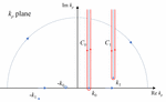
Consider the integral in the complex plane shown in Figure 2. The horizontal axis is the real axis, while the vertical axis is the image axis.

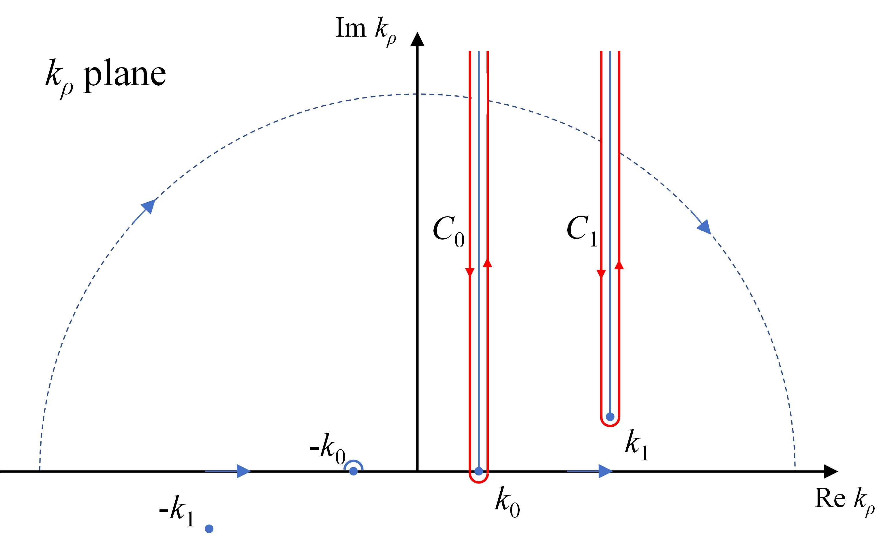
Fig. 2. The $k_{\rho }$ plane.

Extending the integration path to the whole real axis and using the Cauchy theorem, the integration path is deformed to C${}_{\mathrm{0}}$ and C${}_{\mathrm{1}}$ as follows:

	${\displaystyle \frac{1}{2}}\left(k_1^2-k_0^2\right)F_{1z}^r(\rho ,x)$	(15)
	$={\displaystyle {\int }_{-\mathrm{\infty }}^{\mathrm{\infty }}}\mathit{d}{k}_{\rho }{k}_{\rho }^3{k}_{0z}\left[e^{i\left(k_{0z}+\sqrt{k_1^2-k_0^2}\right)x}-e^{i{k}_{1z}x}\right]H_0^{\left(1\right)}\left(k_{\rho }\rho \right)$
	$=\underset{C_0+C_1}{\int }d{k}_{\rho }{k}_{\rho }^3{k}_{0z}\left[e^{i\left(k_{0z}+\sqrt{k_1^2-k_0^2}\right)x}-e^{i{k}_{1z}x}\right]H_0^{\left(1\right)}\left(k_{\rho }\rho \right).$

Denote $f\left(k_{\rho }\right)=k_{\rho }^3{k}_{0z}\left[e^{i\left(k_{0z}+\sqrt{k_1^2-k_0^2}\right)x}-e^{i{k}_{1z}x}\right]H_0^{\left(1\right)}\left(k_{\rho }\rho \right)$, and it has five branch points at $k_{\rho }=0\pm k_0\pm k_1$. The branch points and the related branch cuts are also depicted in Figure 2. The branch cuts are parallel to the image axis. While passing the branch points, the integration path should have appropriate indentations as shown in Figure 2.

Using the double saddle point method [10], the integrals along the path C${}_{\mathrm{0}}$ and C${}_{\mathrm{1}}$ can be expanded with asymptotic series, respectively

	${\displaystyle {\int }_{C_0}}f\left(k_{\rho }\right)\mathit{d}{k}_{\rho }\sim e^{i{k}_0\rho }\left({\displaystyle \frac{A_3}{{\rho }^3}}+{\displaystyle \frac{A_4}{{\rho }^4}}+{\displaystyle \frac{A_5}{{\rho }^5}}+\mathrm{\cdots }\right),$	(16)
	${\displaystyle {\int }_{C_1}}f\left(k_{\rho }\right)\mathit{d}{k}_{\rho }\sim e^{i{k}_1\rho }\left({\displaystyle \frac{B_2}{{\rho }^2}}+{\displaystyle \frac{B_3}{{\rho }^3}}+{\displaystyle \frac{B_4}{{\rho }^4}}+\mathrm{\cdots }\right).$

$A_n$ and $B_n$ are constants determined by the Taylor series of $f\left(k_{\rho }\right)$ at $k_{\rho }=k_0$ and $k_{\rho }=k_1$. For example, the $A_3$ term is

$$A_3=\frac{4k_0^2}{i\pi }\left[4e^{i\sqrt{k_1^2-k_0^2}x}-\frac{3k_0^2{x}^2}{2}-\frac{3i{k}_0^{2}x}{2\sqrt{k_1^2-k_0^2}}-4\right].$$

(17)

The coefficients are lengthy but easy to be obtained by the commercial software Mathematica. What should be emphasized is that the exact forms of the coefficients $A_n$ and $B_n$ are not important in the realistic approximation because the residual integrals are to be neglected. The series is just used while proving the effectiveness of our method.

Since $Im\left(k_1\right)>0$, $e^{i{k}_1\rho }=o\left(1/r^n\right)$ ($n\in Z_{+}$), it can be deduced from eqn (16) that only the integral on the path $C_0$ should be taken into consideration as $\rho \to \mathrm{\infty }$. Therefore,

$${\int }_{C_0+C_1}f\left(k_{\rho }\right)\mathit{d}{k}_{\rho }\sim e^{i{k}_0\rho }\left(\frac{A_3}{{\rho }^3}+\frac{A_4}{{\rho }^4}+\frac{A_5}{{\rho }^5}+\mathrm{\cdots }\right).$$

(18)

Combining eqn (15) and (18), the asymptotic series of $F_{1z}^r(\rho ,x)$ can be written as

$$F_{1z}^r(\rho ,x)\sim \frac{e^{i\left(x\sqrt{k_1^2-k_0^2}+k_0\rho \right)}}{2\left(k_1^2-k_0^2\right)}\left(\frac{A_3}{{\rho }^3}+\frac{A_4}{{\rho }^4}+\frac{A_5}{{\rho }^5}+\mathrm{\cdots }\right).$$

(19)

According to eqn (14)–(19), the relative error $e_r$ between $F_{1z}(\rho ,x)$ and $F_{1z}^e(\rho ,x)$ is found to be

$e_r$	$={\displaystyle \frac{F_{1z}(\rho ,x)-F_{1z}^e(\rho ,x)}{F_{1z}(\rho ,x)}}$	(20)
	$={\displaystyle \frac{o\left(1/{\rho }^2\right)}{o\left(1/{\rho }^2\right)+\mathrm{o}\left(1/{\rho }^2\right)+A/{\rho }^2}}=o\left(1\right).$

The above equation means $e_r\to 0$ as $\rho \to \mathrm{\infty }$, so $F_{1z}^e(\rho ,x)$ is a good approximation of $F_{1z}(\rho ,x)$. In other words, $F_{1z}^r(\rho ,x)$ could be neglected in $F_{1z}(\rho ,x)$ which confirms our previous observation.

It can be checked from (13) and (19) that the lowest negative order term $1/{\rho }^2$ is extracted and included in the explicit expression $F_{1z}^e(\rho ,x)$, making it a more accurate approximate expression for the lateral wave at large radial distance. $F_{\rho }(\rho ,z)$ and $F_{\varphi }(\rho ,x)$ can be dealt with in a similar way

$$\begin{array}{ccc}\hfill F_{\rho }(\rho ,x)& \hfill =\hfill & F_{1\rho }^e(\rho ,x)+F_{1\rho }^r(\rho ,x),\hfill \\ \hfill F_{\varphi }(\rho ,x)& \hfill =\hfill & F_{1\varphi }^e(\rho ,x)+F_{1\varphi }^r(\rho ,x).\hfill \end{array}$$

(21)

$F_{1\rho }^e(\rho ,x)$, $F_{1\varphi }^e(\rho ,x)$, $F_{1\rho }^r(\rho ,x)$, and $F_{1\varphi }^r(\rho ,x)$ are defined by eqn (22) and (23). Due to the term-wise differentiable property of the asymptotic series of the residual integrals [10], it can be proved that $F_{1\rho }^r(\rho ,x)$ and $F_{1\varphi }^r(\rho ,x)$ could also be neglected when $\rho$ is large enough.

$$\{\begin{array}{c}{F}_{1\rho }^e(\rho ,x)=\frac{\rho }{2i\left(k_1^2-k_0^2\right)}\hfill \\ \times \frac{\partial }{\partial x}\left[I_2(\rho ,x,k_1)-e^{i\sqrt{k_1^2-k_0^2}x}{I}_2(\rho ,x,k_0)\right],\hfill \\ F_{1\varphi }^e(\rho ,x)=\frac{1}{k_1^2-k_0^2}\hfill \\ \times \left[I_2(\rho ,x,k_1)-e^{i\sqrt{k_1^2-k_0^2}x}{I}_2(\rho ,x,k_0)\right].\hfill \end{array}$$

(22)

$$\{\begin{array}{c}{F}_{1\rho }^r(\rho ,x)=\frac{1}{i\left(k_1^2-k_0^2\right)}\times \frac{{\partial }^2}{\partial x\partial \rho }{\int }_0^{\mathrm{\infty }}\mathit{d}{k}_{\rho }{k}_{\rho }{k}_{0z}\hfill \\ \left[e^{i{k}_{1z}x}-e^{i\left(k_{0z}+\sqrt{k_1^2-k_0^2}\right)x}\right]J_0\left(k_{\rho }\rho \right),\hfill \\ F_{1\varphi }^r(\rho ,x)=\frac{1}{k_1^2-k_0^2}\times \frac{\partial }{\partial \rho }{\int }_0^{\mathrm{\infty }}\mathit{d}{k}_{\rho }{k}_{\rho }{k}_{0z}\hfill \\ \left[e^{i{k}_{1z}x}-e^{i\left(k_{0z}+\sqrt{k_1^2-k_0^2}\right)x}\right]J_0\left(k_{\rho }\rho \right).\hfill \end{array}$$

(23)

Hence, the explicit expressions of the lateral waves in the sea are

	$H_{1z}^{\mathrm{lat}}={\displaystyle \frac{M}{2\pi i}}{F}_{1z}^e(\rho ,d-z),$	(24)
	$H_{1\rho }^{\mathrm{lat}}={\displaystyle \frac{M}{2\pi }}{F}_{1\rho }^e(\rho ,d-z),$
	$E_{1\varphi }^{\mathrm{lat}}={\displaystyle \frac{\omega {\mu }_{1}M}{2\pi }}{F}_{1\varphi }^e(\rho ,d-z).$

Thus, combining eqn (5) and (24), the EM field in the sea can be expressed with explicit expressions.

D. EM fields in the air

The nonzero EM field components in the air ($z>0$) can be expressed as

	$H_{0z}={\displaystyle \frac{M}{2\pi i}}{\displaystyle {\int }_0^{\mathrm{\infty }}}\mathit{d}{k}_{\rho }{\displaystyle \frac{k_{\rho }^3}{k_{1z}+k_{0z}}}{e}^{i{k}_{1z}d}{e}^{i{k}_{0z}z}{J}_0\left(k_{\rho }\rho \right),$	(25)
	$H_{0\rho }=-{\displaystyle \frac{M}{2\pi }}{\displaystyle {\int }_0^{\mathrm{\infty }}}\mathit{d}{k}_{\rho }{\displaystyle \frac{k_{0z}{k}_{\rho }^2}{k_{1z}+k_{0z}}}{e}^{i{k}_{1z}d}{e}^{i{k}_{0z}z}{J}_1\left(k_{\rho }\rho \right),$
	$E_{0\varphi }={\displaystyle \frac{\omega {\mu }_{0}M}{2\pi }}{\displaystyle {\int }_0^{\mathrm{\infty }}}\mathit{d}{k}_{\rho }{\displaystyle \frac{k_{\rho }^2}{k_{1z}+k_{0z}}}{e}^{i{k}_{1z}d}{e}^{i{k}_{0z}z}{J}_1\left(k_{\rho }\rho \right).$

Conventionally, there is no need to decompose the components of the EM fields in the air like in the sea. The components themselves constitute the lateral wave in the air. Under this circumstance, the problem is a little different from that in the sea because the exponential factors contain both $k_{1z}$ and $k_{0z}$. Nevertheless, the core idea can be applied to extract the dominant term for the lateral wave from the integrals and abandon the residual integrals.

Denote that

	$F_{0z}(\rho ,z,d)={\displaystyle {\int }_0^{\mathrm{\infty }}}\mathit{d}{k}_{\rho }{\displaystyle \frac{k_{\rho }^3}{k_{1z}+k_{0z}}}{e}^{i{k}_{1z}d}{e}^{i{k}_{0z}z}{J}_0\left(k_{\rho }\rho \right),$	(26)
	$F_{0\rho }(\rho ,z,d)={\displaystyle {\int }_0^{\mathrm{\infty }}}\mathit{d}{k}_{\rho }{\displaystyle \frac{k_{0z}{k}_{\rho }^2}{k_{1z}+k_{0z}}}{e}^{i{k}_{1z}d}{e}^{i{k}_{0z}z}{J}_1\left(k_{\rho }\rho \right),$
	$F_{0\varphi }(\rho ,z,d)={\displaystyle {\int }_0^{\mathrm{\infty }}}\mathit{d}{k}_{\rho }{\displaystyle \frac{k_{\rho }^2}{k_{1z}+k_{0z}}}{e}^{i{k}_{1z}d}{e}^{i{k}_{0z}z}{J}_1\left(k_{\rho }\rho \right).$

Now, the lateral wave in the air can be written as

	$H_{0z}={\displaystyle \frac{M}{2\pi i}}{F}_{0z}(\rho ,z,d),$	(27)
	$H_{0\rho }={\displaystyle \frac{M}{2\pi }}{F}_{0\rho }(\rho ,z,d),$
	$E_{0\varphi }={\displaystyle \frac{M\omega {\mu }_0}{2\pi }}{F}_{0\varphi }(\rho ,z,d).$

Recalling eqn (18), the integral on C${}_{\mathrm{1}}$ plays an insignificant role in the lateral wave when $\rho$ is large. To extract the dominant part from the integral expression of the lateral wave, we only need to make the lowest negative power term of the asymptotic series of the integrals on the integration path C${}_{\mathrm{0}}$vanish like (16). To achieve this, the extraction is performed as follows:

	$F_{0z}(\rho ,z,d)=F_{0z}^e(\rho ,z,d)+F_{0z}^r(\rho ,z,d),$	(28)
	$F_{0\rho }(\rho ,z,d)=F_{0\rho }^e(\rho ,z,d)+F_{0\rho }^r(\rho ,z,d),$
	$F_{0\varphi }(\rho ,z,d)=F_{0\varphi }^e(\rho ,z,d)+F_{0\varphi }^r(\rho ,z,d).$

Related functions in eqn (28) are defined in eqn (29) and (30). It can be verified that the lowest negative order terms vanish in the asymptotic series of the residual integrals. Hence, for large radial distance, all the residual integrals $F_{0z}^r(\rho ,z,d)$, $F_{0\rho }^r(\rho ,z,d)$, and $F_{0\varphi }^r(\rho ,z,d)$ can be neglected, and the EM fields in the air can be represented by the explicit expressions as shown in eqn (31).

$$\{\begin{array}{c}{F}_{0z}^e(\rho ,z,d)=\frac{1}{i\left(k_1^2-k_0^2\right)}\left(\frac{\partial }{\partial d}-\frac{\partial }{\partial z}\right)\hfill \\ \left[I_3(\rho ,d,k_1)+e^{i\sqrt{k_1^2-k_0^2}d}{I}_3(\rho ,z,k_0)\right],\hfill \\ F_{0\rho }^e(\rho ,z,d)=\frac{1}{k_1^2-k_0^2}\frac{\partial }{\partial z}\left(\frac{\partial }{\partial d}-\frac{\partial }{\partial z}\right)\frac{\partial }{\partial \rho }\hfill \\ \left[I_4(\rho ,d,k_1)+e^{i\sqrt{k_1^2-k_0^2}d}{I}_4(\rho ,z,k_0)\right],\hfill \\ F_{0\varphi }^e(\rho ,z,d)=\frac{i}{\left(k_1^2-k_0^2\right)}\left(\frac{\partial }{\partial d}-\frac{\partial }{\partial z}\right)\frac{\partial }{\partial \rho }\hfill \\ \left[I_4(\rho ,d,k_1)+e^{i\sqrt{k_1^2-k_0^2}d}{I}_4(\rho ,z,k_0)\right].\hfill \end{array}$$

(29)

$$\{\begin{array}{c}{F}_{0z}^r(\rho ,z,d)=\frac{1}{i\left(k_1^2-k_0^2\right)}\left(\frac{\partial }{\partial d}-\frac{\partial }{\partial z}\right){\int }_0^{\mathrm{\infty }}\mathit{d}{k}_{\rho }{k}_{\rho }^3\hfill \\ \left(e^{i{k}_{1z}d}-e^{i\sqrt{k_1^2-k_0^2}d}\right)\left(e^{i{k}_{0z}z}-1\right)J_0\left(k_{\rho }\rho \right),\hfill \\ F_{0\rho }^r(\rho ,z,d)=\frac{1}{k_1^2-k_0^2}\frac{\partial }{\partial z}\left(\frac{\partial }{\partial d}-\frac{\partial }{\partial z}\right)\frac{\partial }{\partial \rho }{\int }_0^{\mathrm{\infty }}\mathit{d}{k}_{\rho }{k}_{\rho }\hfill \\ \left(e^{i{k}_{1z}d}-e^{i\sqrt{k_1^2-k_0^2}d}\right)\left(e^{i{k}_{0z}z}-1\right)J_0\left(k_{\rho }\rho \right),\hfill \\ F_{0\varphi }^r(\rho ,z,d)=\frac{i}{\left(k_1^2-k_0^2\right)}\left(\frac{\partial }{\partial d}-\frac{\partial }{\partial z}\right)\frac{\partial }{\partial \rho }{\int }_0^{\mathrm{\infty }}\mathit{d}{k}_{\rho }{k}_{\rho }\hfill \\ \left(e^{i{k}_{1z}d}-e^{i\sqrt{k_1^2-k_0^2}d}\right)\left(e^{i{k}_{0z}z}-1\right)J_0\left(k_{\rho }\rho \right).\hfill \end{array}$$

(30)

	$H_{0z}={\displaystyle \frac{M}{2\pi i}}{F}_{0z}^e(\rho ,z,d),$	(31)
	$H_{0\rho }={\displaystyle \frac{M}{2\pi }}{F}_{0\rho }^e(\rho ,z,d),$
	$E_{0\varphi }={\displaystyle \frac{M\omega {\mu }_0}{2\pi }}{F}_{0\varphi }^e(\rho ,z,d).$

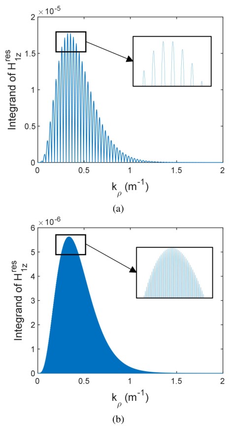
Fig. 3. The comparison of the integrands at (a) $\rho$ = 100 m and (b) $\rho$ = 1000 m.

III. RESULTS

In this section, some numerical results and comparisons are given. First, the VMD is placed in the sea at $d=10$m and the working frequency is $f=50$ Hz. The lateral waves at $z=-0.5$ m and $z=0.5$ m are considered. The results are compared with King’s results and they are in good agreement. Then, the EM fields are calculated when the restriction condition $\left|k_1\right|\gg \left|k_0\right|$ is not satisfied. It can be seen from the numerical results that King’s approximation method could not give accurate results in this situation. Nevertheless, our method could still give the accurate results.

Now consider the VMD placed in the sea at first.

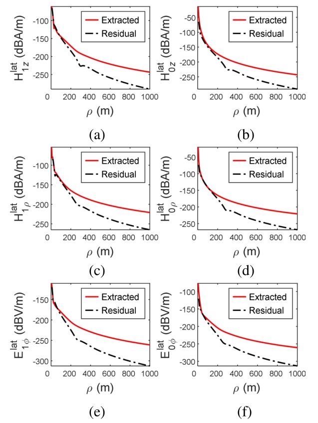
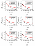
Fig. 4. The comparison of the extracted parts and the residual integrals: (a) $H_{1z}^{\mathrm{lat}}$, (b) $H_{0z}^{\mathrm{lat}}$, (c) $H_{1\rho }^{\mathrm{lat}}$, (b) $H_{0\rho }^{\mathrm{lat}}$, (e) $E_{1\varphi }^{\mathrm{lat}}$, and (f) $E_{0\varphi }^{\mathrm{lat}}$.

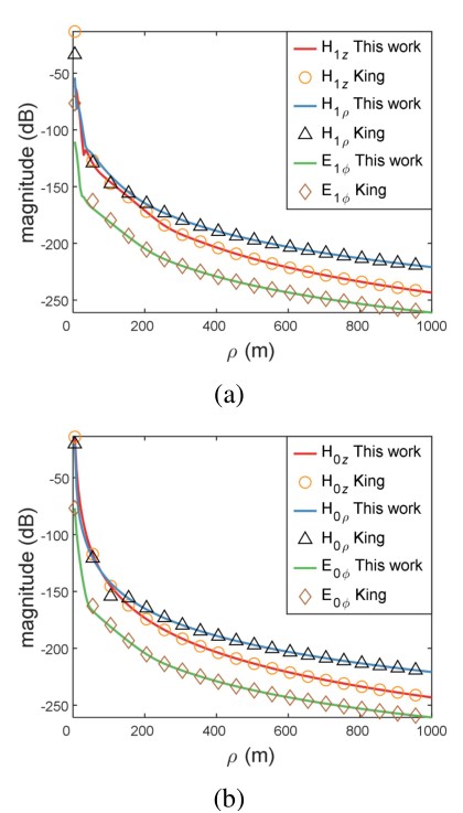
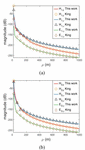
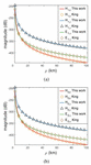
Fig. 5. The comparison of the results within $\rho$ $\mathrm{<}$ 1000 m of our method and King’s method. (a) Field in the sea. (b) Field in the air.

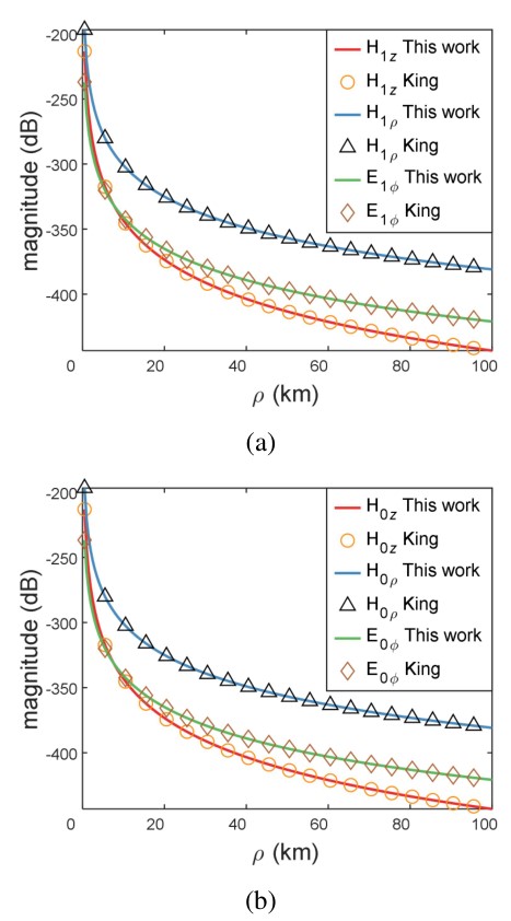
Fig. 6. The comparison of the results within $\rho$ $\mathrm{<}$ 100 km of our method and King’s method. (a) Field in the sea. (b) Field in the air.

Figure 3 shows the comparison of the integrands of $H_{1z}^{\mathrm{lat}}$ at different radial distances. It can be observed that the integrands possess rapid oscillations, and the oscillation rate increases with $\rho$. Therefore, the direct numerical evaluation of the integral is inefficient when $\rho$ is large.

In Figure 4, the solid curves represent the modulus of the extracted parts of the field components and the dashed lines represent the corresponding counterpart of residual parts. When $\rho$ exceeds 200 m, the residual integrals become negligible compared with the extracted explicit parts.

The results of our method are also compared with the results obtained by the method of King (refer to Appendix D of [3]). Figure 5 shows the comparison in the range $\rho <1000$ m. The solid lines are the results of our method, and the symbols are the results of King’s method. While $\rho$ is larger than about 200 m, the results of the two methods match very well because the requirement of $\left|k_1\right|\gg \left|k_0\right|$ for King’s method is satisfied in this example.

Figure 6 shows the comparison within $\rho <100$km. It is known that the traditional numerical methods become very inefficient when $\rho$ reaches such a large distance.

Next consider the problem when the restriction condition $\left|k_1\right|\gg \left|k_0\right|$ no longer holds. Specifically, the conductivity of the lower half space is $1\times {10}^{-6}$ S/m and the permittivity of the upper half space is $200{ϵ}_0$ now. The working frequency $f$ is 5.2 kHz and $d=500$ m. The other parameters remain the same.

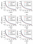
Figure 7 shows the comparison of the results of our method, King’s method, and the direct numerical integration. It can be seen from the figure that the results of our method match very well with the direct numerical integration results, which are made converged with high accuracy but very time-consuming. However, the field components obtained by King’s method could not give accurate results as shown in Figure 7.

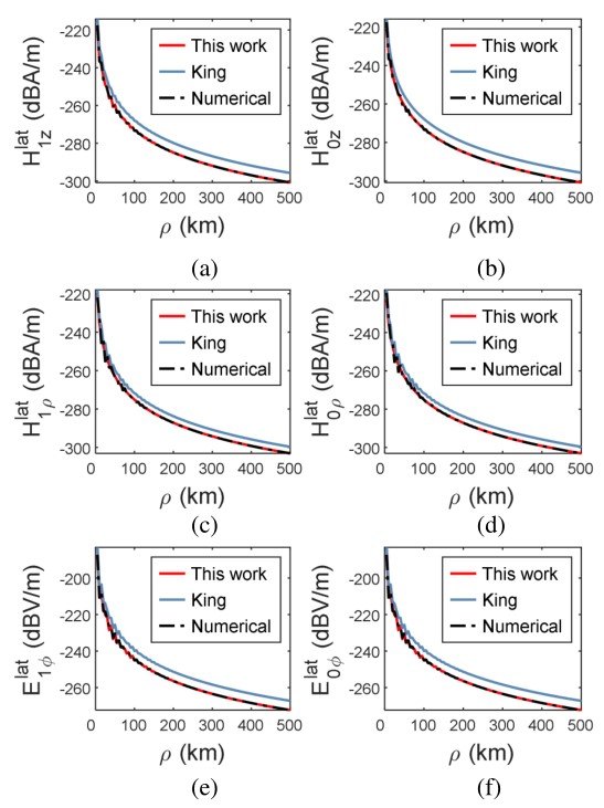
Fig. 7. The comparison of the results obtained by different methods: (a) $H_{1z}^{\mathrm{lat}}$, (b) $H_{0z}^{\mathrm{lat}}$, (c) $H_{1\rho }^{\mathrm{lat}}$, (b) $H_{0\rho }^{\mathrm{lat}}$, (e) $E_{1\varphi }^{\mathrm{lat}}$, and (f) $E_{0\varphi }^{\mathrm{lat}}$.

IV. CONCLUSION

In this paper, a method for efficiently evaluating the fields of a VMD in a dissipative half space is proposed. Dominant explicit formulae for nonzero field components are extracted from their integral expressions. The residual integrals are negligible for large radial distance. Since no numerical integration is needed, this method is efficient for calculating the far fields. Besides, it has no restriction on the parameters of the media; so it has broader application scope than the King’s method when dealing with different problems.

ACKNOWLEDGMENT

This work is supported by Shanghai Academy of Spaceflight Technology (SAST)—Shanghai Jiao Tong University advanced aerospace technology joint research center funded projects under Grant USCAST2019-21.

REFERENCES

[1] A. N. Sommerfeld, “Propagation of waves in wireless telegraphy,” Ann. Phys. (Leipzig), vol. 28, pp. 665-737, 1909.

[2] J. Zenneck, “Propagation of plane EM waves along a plane conducting surface,” Ann. Phys.(Leipzig), vol. 23, no. 1, pp. 907, 1907.

[3] R. W. King, M. Owens, and T. T. Wu, Lateral Electromagnetic Waves: Theory and Applications to Communications, Geophysical Exploration, and Remote Sensing, 1st ed. Springer-Verlag Inc., New York, USA, 1992.

[4] V. A. Houdzoumis, “Lateral waves over planar earth: a validity check of a proposed solution,” IEEE Transactions on Antennas and Propagation., vol. 57, no. 2, pp. 567-572, 2009.

[5] H. Wang, Y. Yang, K. Yang, and Y. Ma, “Verification and evaluation of lateral wave propagation in marine environment,” IEEE Antennas and Wireless Propagation Letters., vol. 19, no. 12, pp. 2413-2417, 2020.

[6] J. Zou, T. N. Jiang, J. B. Lee, and S. H. Chang, “Fast calculation of the electromagnetic field by a vertical electric dipole over a lossy ground and its application in evaluating the lightning radiation field in the frequency domain,” IEEE Transactions on Electromagnetic Compatibility., vol. 52, no. 1, pp. 147-154, 2010.

[7] K. A. Norton, “The propagation of radio waves over the surface of the earth and in the upper atmosphere,” Proceedings of the Institute of Radio Engineers., vol. 25, no. 9, pp. 1203-1236, 1937.

[8] R. W. P. King, “Lateral electromagnetic waves from a horizontal antenna for remote sensing in the ocean,” IEEE Transactions on Antennas and Propagation., vol. 37, no. 10, pp. 1250-1255, 1989.

[9] A. V. Osipov and S. A. Tretyakov, Electromagnetic Scattering Theory with Applications, 1st ed. John Wiley & Sons, Inc., Chichester, West Sussex, 2017.

[10] A. Baños, Dipole Radiation in the Presence of a Conducting Half-Space, 1st ed. Pergamon Press Inc., 1966.

[11] M. Siegel and R. King, “Radiation from linear antennas in a dissipative half-space,” IEEE Trans. Antennas Propagat., vol. 19, no. 4, pp. 477-485, Jul. 1971.

[12] M. Siegel and R. King, “Electromagnetic propagation between antennas submerged in the ocean,” IEEE Trans. Antennas Propagat., vol. 21, no. 4, pp. 507-513, Jul. 1973.

[13] L. Shen, R. W. King, and R. Sorbello, “Measured field of a directional antenna submerged in a lake,” IEEE Trans. Antennas Propagat., vol. 24, no. 6, pp. 891-894, Nov. 1976.

[14] W. C. Chew, Waves and Fields in Inhomogeneous Media, 1st ed. IEEE Press Inc., New York, USA, 1990.

[15] K. A. Michalski and D. Zheng, “Electromagnetic scattering and radiation by surfaces of arbitrary shape in layered media. I. theory,” IEEE Trans. Antennas Propagat., vol. 38, no. 3, pp. 335-344, Mar. 1990.

[16] P. YlaOijala, M. Taskinen, and J. Sarvas, “Multilayered media Green’s functions for MPIE with general electric and magnetic sources by the hertz potential approach - abstract,” Progress In Electromagnetics Research, vol. 33, no. 7, pp. 141-165, Apr. 2001.

[17] W. C. Chew, J. S. Xiong, and T. J. Cui, “The layered medium Green’s function - a new look,” Microwave and Optical Technology Letters, vol. 31, no. 4, pp. 252-255, Oct. 2001.

[18] K. A. Michalski, “Extrapolation methods for Sommerfeld integral tails,” IEEE Trans. Antennas Propagat., vol. 46, no. 10, pp. 1405-1418, Oct. 1998.

[19] J. Mosig, “The weighted averages algorithm revisited,” IEEE Trans. Antennas Propagat., vol. 60, no. 4, pp. 2011-2018, Jan. 2012.

[20] Y. Hua and T. K. Sarkar, “Generalized pencil-of-function method for extracting poles of an EM system from its transient response,” IEEE Trans. Antennas Propagat., vol. 37, no. 2, pp. 229-234, Feb. 1989.

[21] M. I. Aksun and G. Dural, “Clarification of issues on the closed-form Green’s functions in stratified media,” IEEE Trans. Antennas Propagat., vol. 53, no. 11, pp. 3644-3653, Nov. 2005.

[22] M. Yuan, T. K. Sarkar, and M. Salazar-Palma, “A direct discrete complex image method from the closed-form Green’s functions in multilayered media,” IEEE Antennas Wireless Propog. Lett, vol. 54, no. 3, pp. 1025-1032, Mar. 2006.

[23] A. Alparslan, M. I. Aksun, and K. A. Michalski, “Closed-form Green’s functions in planar layered media for all ranges and materials,” IEEE Antennas Wireless Propog. Lett, vol. 58, no. 3, pp. 602-613, Mar. 2010.

[24] J. A. Kong, Electromagnetic Wave Theory, 1st ed. Jonn Wiley & Sons Inc., New Jersey, USA, pp. 220-325, 1986.

BIOGRAPHIES

Hongyun Deng received the B.S. degree from Shanghai Jiao Tong University, Shanghai, China, in 2020. He is currently working toward the M.S. degree in electronic engineering with Shanghai Jiao Tong University. His research interests include computational electromagnetics and electromagnetic theory.

Gaobiao Xiao received the B.S. degree from Huazhong University of Science and Technology, Wuhan, China, in 1988, the M.S. degree from the National University of Defense Technology, Changsha, China, in 1991, and the Ph.D. degree from Chiba University, Chiba, Japan, in 2002. He has been a faculty member since 2004 with the Department of Electronic Engineering, Shanghai Jiao Tong University, Shanghai, China. His research interests are computational electromagnetics, coupled thermo-electromagnetic analysis, microwave filter designs, fiber-optic filter designs, phased array antennas, and inverse scattering problems.

Shifeng Huang received the B.S. and M.S. degrees from Wuhan University, Wuhan, China, in 2014 and 2017, respectively. He is currently working toward the Ph.D. degree in electronic engineering with Shanghai Jiao Tong University, Shanghai, China. His current research interests include computational electromagnetics and its application in electromagnetic compatibility and scattering problems.

ACES JOURNAL, Vol. 36, No. 11, 1393–1400.
doi: 10.13052/2021.ACES.J.361101
© 2021 River Publishers

Abstract

I. INTRODUCTION

II. FORMULATION

A. Model

B. Integral expressions of the EM fields

C. EM fields in the sea

D. EM fields in the air

III. RESULTS

IV. CONCLUSION

ACKNOWLEDGMENT

REFERENCES

BIOGRAPHIES