Linear Antenna Array Synthesis by Modified Seagull Optimization Algorithm
Erhan Kurt, Suad Basbug, and Kerim Guney
1Department of Electrical and Electronics Engineering,
Nuh Naci Yazgan University, Kayseri, 38170, Turkey
2Department of Electrical and Electronics Engineering,
Nevsehir Haci Bektas Veli University, Nevsehir, 50300, Turkey
E-Mail: ekurt@nny.edu.tr; kguney@nny.edu.tr ; suad@nevsehir.edu.tr
Submitted On: October 20, 2021; Accepted On: December 12, 2021
Abstract
This paper presents a study of linear antenna array (LAA) synthesis with a seagull optimization algorithm (SOA) to achieve radiation patterns having low maximum sidelobe levels (MSLs) with and without nulls. The SOA is a new optimization technique based on the moving and attacking behaviors of the seagull in the nature. In this study, the original mathematical model of SOA is modified by compensating the exploration and exploitation features to improve the optimization performance. The optimization ability of the modified SOA (MSOA) is tested with seven numerical examples of LAA. In the first three examples, the amplitude values of the array elements are optimized by MSOA whereas the element position values are calculated by MSOA for the last four examples. The numerical results obtained by MSOA are compared with those of different algorithms from the literature. The results reveal that MSOA algorithm is very good at optimizing antenna array parameters to obtain a desired radiation pattern. Additionally, it is seen that MSOA finds better results than the compared algorithms in terms of MSL and single and multiple null depth levels (NDLs). The contribution of the modification of MSOA is shown with a convergence curve to compare with the original one.
Index Terms: antenna array synthesis, linear antenna arrays, maximum sidelobe level, null depth level, seagull optimization algorithm.
I. INTRODUCTION
Antenna arrays are widely used in many communication and radar systems to improve the quality of the signal [1]. The quality of antenna array design significantly effects the performance of these array systems. In recent years, a lot of research has been carried out on the design of antenna arrays to achieve desired radiation pattern synthesis. These parameters are mainly amplitude, phase, and position values of array elements. From this perspective, calculating proper array parameters is an optimization problem. Therefore, many optimization methods have been used to obtain the desired antenna array radiation pattern. Modifications on the radiation pattern are performed for different purposes. Maximum sidelobe level (MSL) reductions are basically used to diminish the negative effect of the electromagnetic pollution. Additionally, the radiated power can be better focused on the main beam direction with the help of sidelobe reduction. Placing nulls on the radiation pattern are generally used to prevent interferences caused by unwanted signals received from other communication systems.
There are several different geometrical structures of antenna arrays used in the wireless systems such as linear [2, 3, 4, 5, 6, 7, 8, 9, 10, 11, 12], circular [13, 14, 15, 16, 17, 18], elliptical [19, 20, 21], and planar antenna arrays [22, 24]. Linear antenna arrays (LAAs) are very common geometry among the array systems. Several antenna elements are placed in a straight line for this geometry. Because of its simple structure, LAAs are used in a wide range of applications. Hence, the synthesis problem of LAA has received remarkable attention throughout the years. Different optimization methods such as grey wolf optimizer (GWO) [2], moth-flame optimization (MFO) [3], ant lion optimization (ALO) [4], biogeography-based optimization (BBO)[5], tabu search algorithm (TSA) [6], memetic algorithm (MA) [6], genetic algorithm (GA) [6], fitness-adaptive differential evolution algorithm (FiADE) [7], particle swarm optimization (PSO) [7, 8], harmony search algorithm (HSA) [9], backtracking search algorithm (BSA) [10], comprehensive learning particle swarm optimizer (CLPSO) [11], and mean variance mapping optimization (MVMO) [12] have been proposed and employed to solve these synthesis problems. GWO is used to obtain an optimal pattern synthesis of LAA with a reduced MSL and nulls in the desired directions [2]. The side lobes of two LAAs with different sizes are suppressed by MFO algorithm [3]. Sidelobe reduction and null placement are also carried out by means of ALO evolutionary algorithm in [4]. BBO is employed in [5] to achieve an optimum pattern synthesis with low MSLs by using amplitude as well as phase and position values of array elements. Cengiz and Tokat [6] have employed TSA, MA, and GA to synthesis three LAAs with different number of array elements. FiADE by Chowdhury et al. [7], which is a modified version of the classical DE algorithm, is also used for LAA. The element positions of the LAA elements are determined by using PSO algorithm to get a low MSL and null placement [8]. HSA is also employed to obtain lower MSLs and deeper null levels [9]. Guney and Durmus [10] have used BSA for pattern nulling of LAA. CLPSO, an improved variant of PSO, is employed by Goudos et al. to optimize three different LAAs [11], and MVMO has been applied to LAA synthesis by Guney and Basbug [12].
This paper presents a simple and effective method using the seagull optimization algorithm (SOA) to design an LAA by optimizing only the amplitude and position values of the antenna array elements. Generally, variable attenuators are used to control amplitude values of the array elements in practice. A symmetrical linear array ensures cheaper practical implementations and less computational effort for calculations. If the design is desired to be dynamic, mechanical driving systems are needed to move antenna array elements for the position-only control techniques. The SOA is a novel bio-inspired metaheuristic algorithm proposed by Dhiman and Kumar [25]. The simple structure of SOA with few parameters makes it applicable to different engineering problems [26, 27, 28]. Nine well-known optimization algorithms are chosen for different benchmark comparisons with SOA to validate its performance [25]. The algorithms compared with SOA are GA, differential evolution algorithm, PSO, spotted hyena optimizer, multi-verse optimizer, MFO, sine cosine algorithm, GWO, and, gravitational search algorithm [25]. In this paper, a modified version of SOA (MSOA) is employed. The modification is on the step size of SOA that defines the movement behavior of population elements. The original version of SOA has already a linear changing strategy for the parameter of the movement behavior. However, this strategy is limited with a linear decrease. In this paper, a nonlinear changing is proposed to improve search quality of SOA with a better exploration in the early phase of the algorithm and a better exploitation in its later phases. The enhancement that achieved by the modification is shown with two pairs of convergence curve comparisons in the first and second examples.
In this paper, seven different LAA optimization examples are considered. For the first three examples, the amplitude values of LAA are calculated by MSOA to achieve low MSLs. The fourth example includes the optimization of the element positions in the LAA to reduce sidelobe levels. In the last three examples, element positions are determined by MSOA to locate nulls at the desired directions of the radiation pattern. The results of MSOA are compared with those of GWO [2], MFO [3], ALO [4], BBO[5] , MA [6], GA [6], TSA [6], FiADE [7], PSO [8], HSA [9], BSA [10], CLPSO [11], and MVMO [12]. It was shown that MSOA can obtain better results than those of the other compared algorithms.
II. PROBLEM FORMULATION
A symmetrical LAA that consists of even number (2N) isotropic elements is illustrated in Figure 1. The array elements are placed symmetrically along the x-axis. Because of the symmetrical structure, LAA has a symmetrical radiation pattern. The elements placed symmetrically can also reduce the computational cost since it is sufficient to optimize only N elements. The array factor of LAA shown in Figure 1 is given by [1]:
| (1) |
where I and are amplitude and phase of n element, respectively. d is the distance from the array center to the n element. is the scanning angle from broadside and k is the wave number which equals to 2/. In the first three examples of this study, the main purpose is to obtain optimum amplitude values (I) of equally spaced antenna array elements to generate diagrams with low MSL values. For the fourth example, the position values (d) of the array elements are optimized by using MSOA to obtain patterns with low MSL values. In the last three examples, in order to achieve radiation patterns with low MSLs and deep nulls placed in desired directions, the element positions (d) of the antenna arrays with constant excitations are calculated by meansof MSOA.
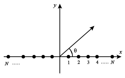
Figure 1: Geometry of a symmetric linear antenna array with elements positioned along x-axis.
A general fitness function is formulated for the all examples as
| (2) |
where f, f, and f functions are used to suppress the MSL, limit the first null beamwidth (FNBW), and place nulls at desired directions, respectively. The function f can be formulated as follows:
| (3) |
where is the first null point in degree on the right side of the main beam. E() is formulated as follows to calculate the values that are greater than the desired MSL (MSL) on the sidelobes:
| (4) |
where
| (5) |
The function f in (2) can be given by
| (6) |
where FNBWand fare the FNBW calculated by MSOA and the desired maximum FNBW, respectively. f in (2) is defined as
| (7) |
where NULL is the desired NDL at the predetermined null angle.
III. METHOD
A. Seagull optimization algorithm
Seagulls are sea birds with many species with different masses and lengths that can live all over the planet. They are omnivores that feed on insects, fish, lizards, frogs, and eggs. The body of seagulls is generally covered with white plumages. Seagulls are highly intelligent animals. They use their intelligence to find and attack the prey. For example, they use breadcrumbs to attract and hunt the fishes. They can also produce sounds like rain to deceive and catch the earthworms. Generally, seagulls live in colonies and there are two most important behaviors for seagulls in terms of swarming. They migrate to other locations and attack their preys together according to a plan. The migration and hunting behaviors of the seagulls are illustrated in Figure 2 [25]. During the migration, the seagulls instinctively consider three different points. First, they try to avoid collision with other population members. Second, each seagull tends to approach the neighbor that has better fitness. Lastly, all seagulls try to sustain their near positions to the seagull which has the best fitness in the flock. When one of the seagulls searches and attacks the prey, it follows a spiral path in the air.
The mathematical model of SOA [25] is based on the pattern of seagull behavior. First of all, the seagulls in the population are distributed randomly as population members through the solution space. The cost function values are calculated for each seagull by using their positions. The cost function as an objective function for the metaheuristic optimization algorithms is the reciprocity of fitness function. In this study, the cost function specialized for antenna array synthesis problems is used.
The migration is a movement of seagulls to find a better hunting place in terms of rich prey populations. The members of seagull population try to avoid a collision with the other members. To model this behavior parameter is used as follows:
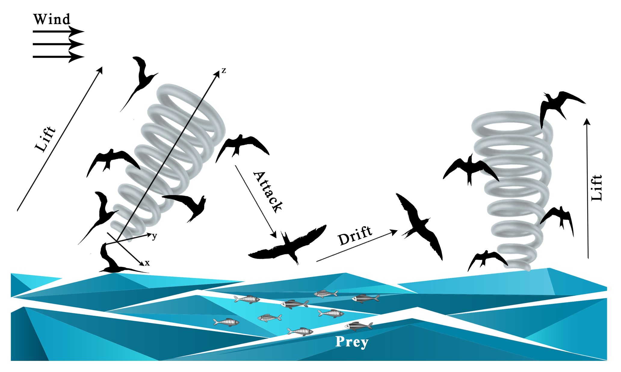
Figure 2: Schematic models of seagulls for their migration and attacking behaviors.
| (8) |
where denotes the position of the seagull that tries to prevent from colliding with other search member. , x, and represent the current position of search member, the current iteration, and the movement behavior of the search member in a given search space, respectively. The parameter is given by
| (9) |
where f is the starting value for the parameter . linearly decreases as iteration progress to 0 as defined in eqn (9). After the collision avoidance mechanism is assured, the search members fly in the direction of the best neighbor. The next position of the search member can be written as
| (10) |
where B, , and represent scaling factor, member having the best cost function value, and current position of search member, respectively. B value is randomized as follows:
| (11) |
where rd is a pseudo random number in [0, 1]. After these processes, the search member changes its position according to the best search member in the population with the following distance formula between the search member and the best member:
| (12) |
The attack is performed by the seagulls to the prey through a spiral-shaped track. This path is modeled as the following formula:
| (13) |
where is the best solution. x’, y’, and z’ in eqn are used to generate the spiral motion:
| (14) |
with
| (15) |
where r, k, u, and v are variable radius of each turn, random number in [0, 2], scaler, and power constants, respectively.
B. Modification on seagull optimization algorithm
This paper also proposes a modification to improve the searching ability of SOA in terms of exploration and exploitation. For this purpose, instead of using eqn (9), parameter in eqn (8) is decreased gradually by tracing a special nonlinear curve defined as follows:
| (16) |
The main idea of this modification is providing a better exploration in the beginning of the iteration process and a finer tunning at the rest of the optimization. In order to achieve this aim, the formulation in eqn (16) is used to provide large steps in the beginning and small steps through the rest of the process as shown in Figure 3. The performance contribution of this modification is validated by comparing the convergence curves of SOA and MSOA solutions for the first example in the following section.
IV. NUMERICAL RESULTS
The results of seven LAA synthesis examples obtained by MSOA are presented in this section. The computer hardware used for the simulations is a Core i5 microprocessor with 16 GB RAM and 2.10 GHz clock speed. The MSOA is implemented on MATLAB version R2020a. The number of iterations for each run is set to 1000. The simulation results for the first three examples and the last four examples are obtained within 35–40 and 50–55 seconds, respectively. The algorithm is run 20 times for each example and the best results are evaluated. The movement behavior () and control frequency (f) parameter of MSOA are set to [2, 0] and 2, respectively. The population size is fixed to 30. Schematic models of seagulls for their migration and attacking behaviors.
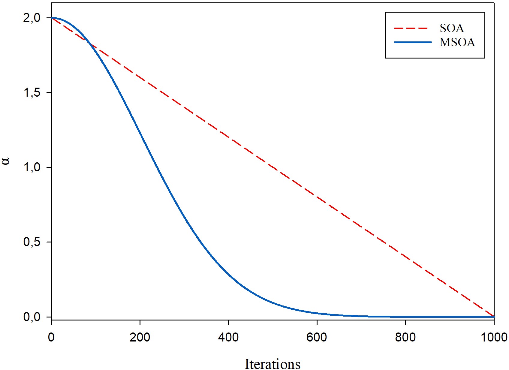
Figure 3: The changes of that models the movement behavior of the search member for the MSOA and SOA.
The synthesis results of MSOA are compared with those of 13 different algorithms, GWO [2], MFO [3], ALO [4], BBO [5], MA [6], GA [6], TSA [6], FiADE [7], PSO [7, 8], HSA [9], BSA [10], CLPSO [11], and MVMO [12]. In the first three examples, MSOA is used to calculate the amplitude values of the array elements to achieve radiation patterns with low MSL values and the results are compared with those of GWO [2], MFO [3], ALO [4], and BBO [5]. For the last four examples, the position values of the array elements are optimized by MSOA and the achieved results are compared with MA [6], GA [6], TSA [6], FiADE [7], PSO [7, 8], HSA [9], BSA [10], CLPSO [11], and MVMO [12].
A. Amplitude only control
In this section, three examples that demonstrate the LAA synthesis with MSL reduction by controlling amplitude-only are given. The phase and interelement position values of the array elements are fixed to = 0 and /2, respectively. The radiation patterns are plotted by using the best amplitude values achieved by 20 different optimization runs.
For the first example, the synthesis of 10-element LAA is considered to achieve low MSL values. The cost function given by eqn (2) is used to optimize with MSOA. Thanks to the array symmetry, it is enough to consider only five elements to optimize their amplitude values. The radiation pattern with low MSL value obtained by MSOA is given in Figure 4. For a comparison, the radiation patterns of GWO [2], MFO [3], and ALO [4] are also given in Figure 4. The MSL results achieved by MSOA are compared with those of GWO [2], MFO [3], ALO [4], and uniform array in Table 1. From the table, it can be said that the MSL value achieved by MSOA is better than those of GWO [2], MFO [3], and ALO [4]. For this example, the convergence curves of the original SOA and MSOA can be seen in Figure 5. It can be concluded from the figure that MSOA can converge faster than the original SOA.
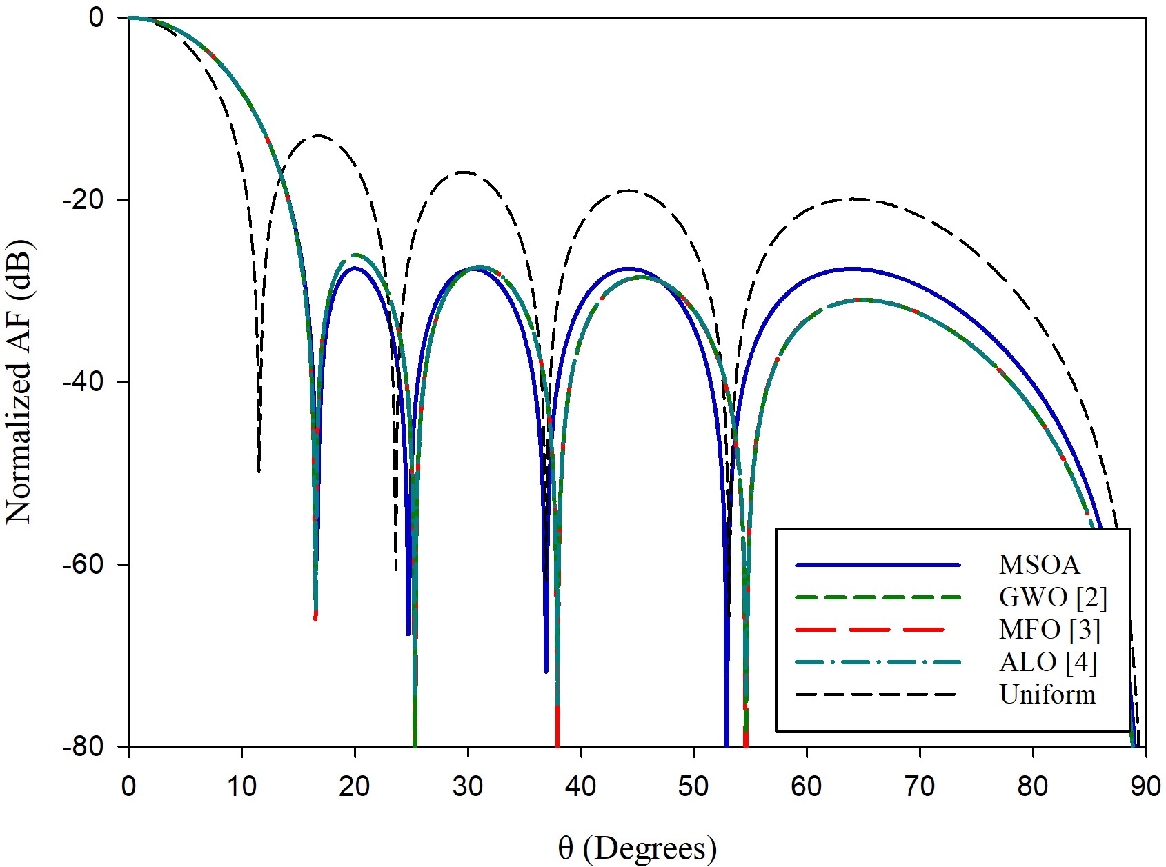
Figure 4: Radiation patterns optimized by MSOA and the compared algorithms GWO [2], MFO [3], and ALO [4] for 10-element LAA.
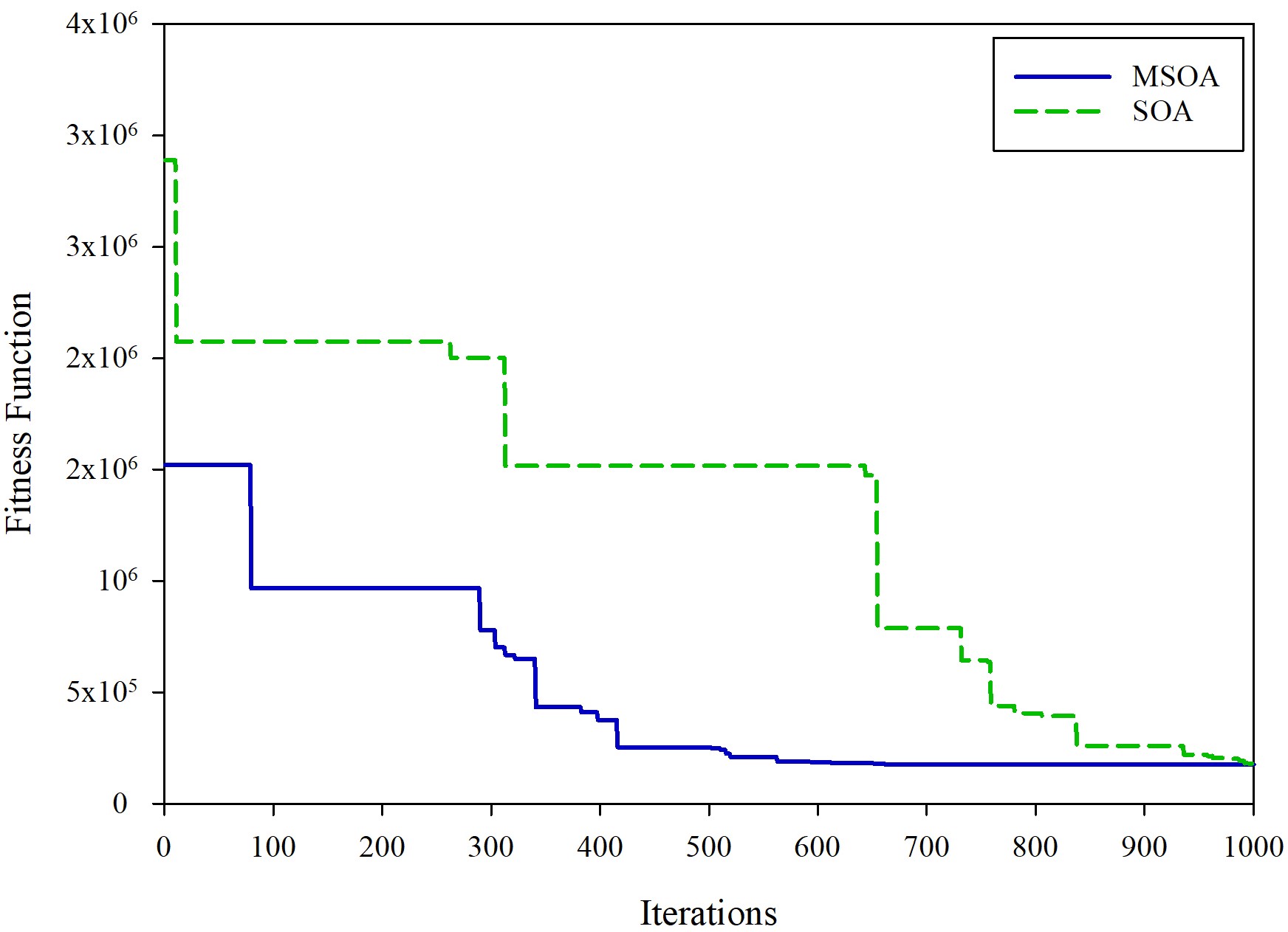
Figure 5: Convergence curve plots of MSOA and SOA for the first example with 10-element LAA.
Table 1: Comparison of the MSL values for 10-element symmetrical LAA design
| Algorithm | MSL (dB) |
|---|---|
| MSOA | –27.52 |
| GWO [2] | –26.05 |
| MFO [3] | –26.07 |
| ALO [4] | –26.08 |
| Uniform | –12.97 |
Table 2: Comparison of the MSL values for 16-element symmetrical LAA design
| Algorithm | MSL (dB) |
|---|---|
| MSOA | –40.65 |
| GWO [2] | –40.50 |
| MFO [3] | –40.25 |
| Uniform | –13.15 |
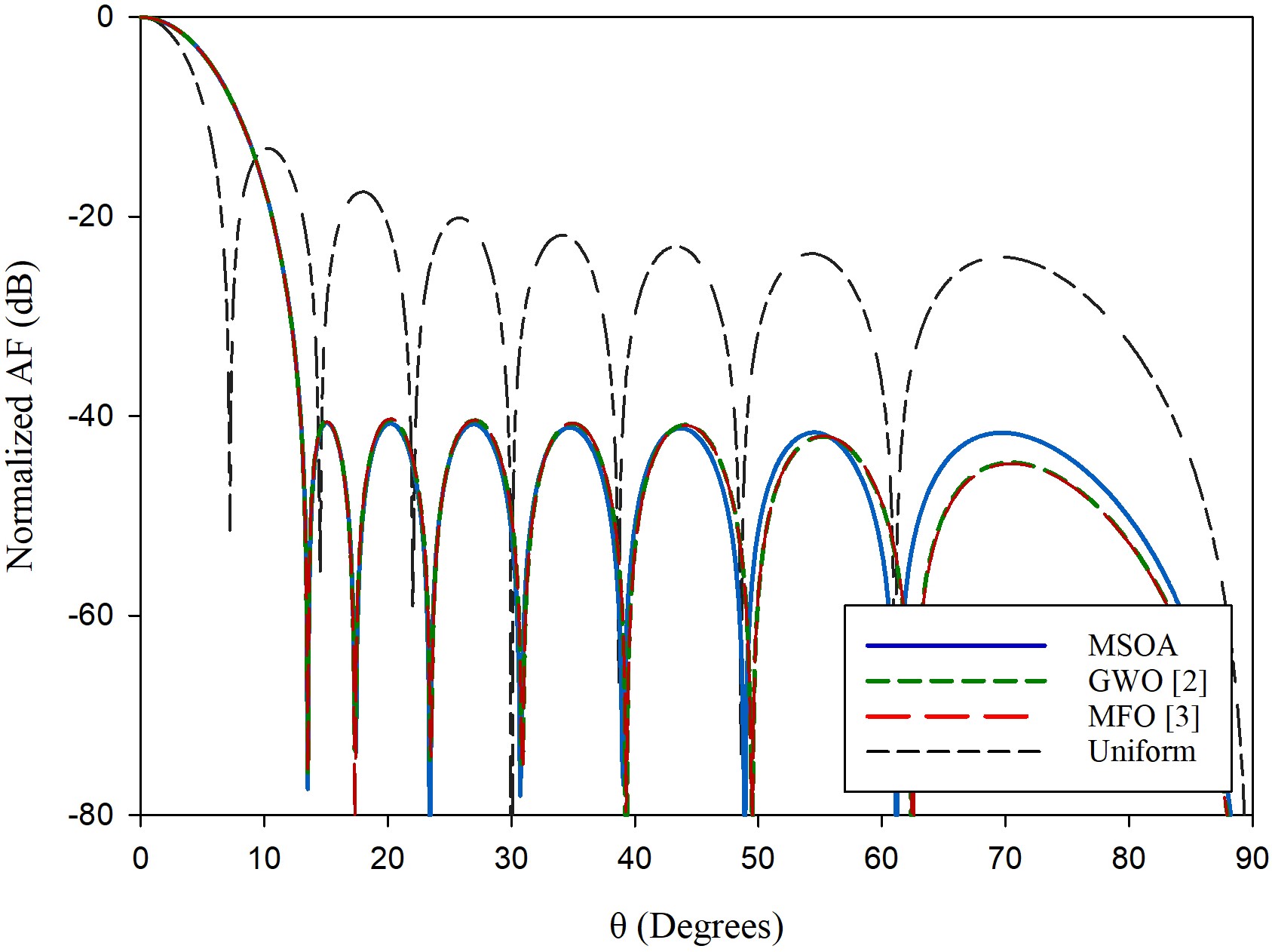
Figure 6: Radiation patterns optimized by MSOA and compared algorithms GWO [2] and MFO [3] for 16-element LAA.
In the second example, a 16-element LAA is optimized by using MSOA method to obtain radiation pattern with low MSL. Figure 6 shows the patterns obtained by MSOA, GWO [2], and MFO [3]. Table 2 presents a comparison between the MSL results achieved by MSOA and those of GWO [2], MFO [3], and uniform array. As shown in Figure 6 and Table 2, the MSL value calculated by MSOA is –40.65 dB which is better than the other compared values. In Figure 7, the convergence curves of the MSOA suggested in this article and original SOA are illustrated. It is very clear from Figure 7 that the MSOA leads to better convergence and that 1000 iterations are needed to find the optimal solutions.
The difference of the third example from the second example is only that the main beam is limited in a fixed region. The third example is designed for a fair comparison with the similar examples from the literature. The main beam is confined as another optimization constraint in addition to the sidelobe restriction. The radiation pattern obtained by MSOA is shown in Figure 8 in comparison with ALO [4] and BBO [5]. The MSL value obtained by MSOA is given in Table 3. In the same table, the MSL results from the literature obtained by other compared algorithms can also be seen. From the table, it can be noted that MSOA has found better MSL value than ALO [4] and BBO [5] algorithms.
The amplitude values of array elements obtained by MSOA for the patterns in Figures 4, 6, and 8 are listed in Table 4.
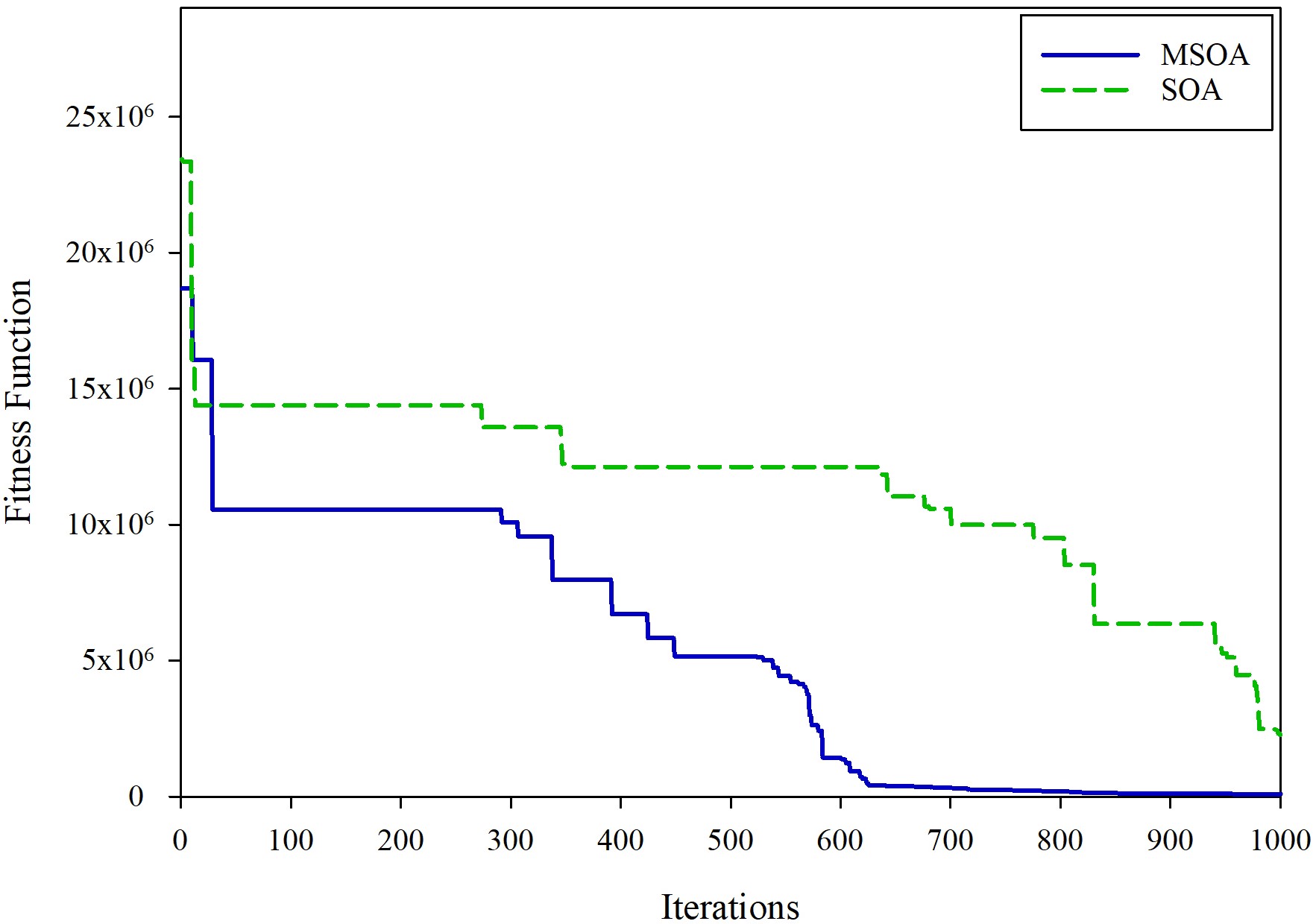
Figure 7: Convergence curve plots of MSOA and SOA for the second example with 16-element LAA.
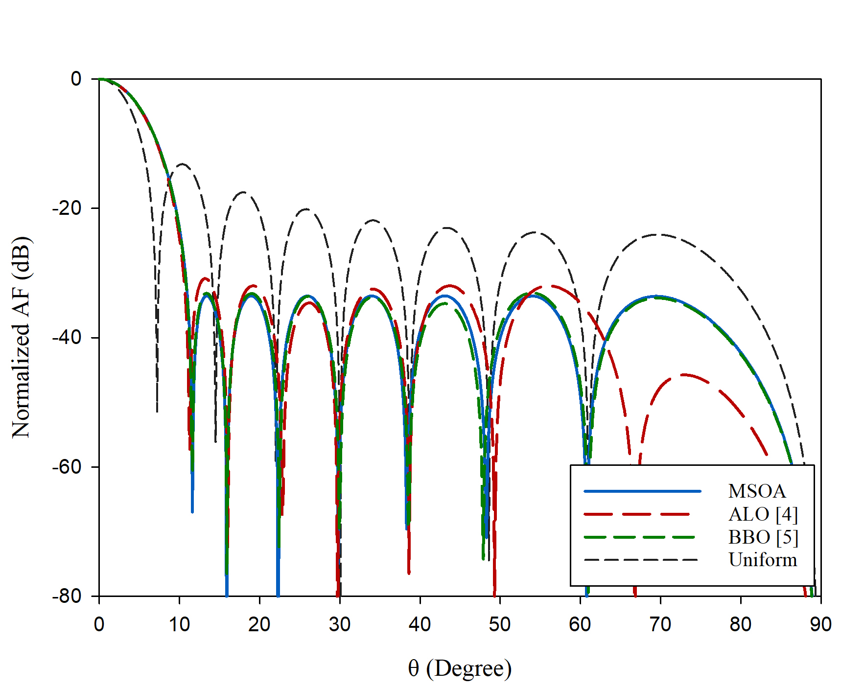
Figure 8: Radiation patterns optimized by MSOA and compared algorithms ALO [4] and BBO [5] for 16-element LAA with constraint FNBW.
Table 3: Comparison of the MSL values for 16-element symmetrical LAA with constraint FNBW
| Algorithm | MSL (dB) |
|---|---|
| MSOA | –33.53 |
| ALO [4] | –30.85 |
| BBO [5] | –33.06 |
Table 4: The element amplitudes (I) for the array patterns given in Figures 4, 6, and 8
| Number of elements | Optimized amplitude values |
|---|---|
| 10 (Figure 4) | [1.0000 0.8887 0.6944 0.4657 0.3154] |
| 16 (Figure 6) | [1.0000 0.9342 0.8121 0.6543 0.4835 0.3220 0.1888 0.1026] |
| 16 (Figure 8) | [1.0000 0.9466 0.8465 0.7125 0.5606 0.4071 0.2681 0.2055] |
B. Position only control
In this section, four examples in which position values of the array elements are adjusted by MSOA are given. The amplitude (I) and phase () values of the array elements are fixed to 1 and 0, respectively.
For the fourth example, 2N = 12 element linear array is considered to achieve a radiation pattern with low MSL values. The cost function given in eqn (2) is used to obtain low MSL by calculating the position values of array elements (d). Figure 9 illustrates the array radiation patterns achieved by using MSOA, TSA [6], MA [6], GA [6], PSO [7], and FiADE [7]. Table 5 presents the MSL values of the radiation patterns calculated by MSOA and the other compared algorithms. From Table 5, it is clear that MSOA has achieved a better MSL value than the other algorithms. It is observed that the physical dimension of antenna array synthesized by MSOA in this work is more compact than those of other antenna arrays optimized by TSA [6], MA [6], GA [6], PSO [7], and FiADE [7].
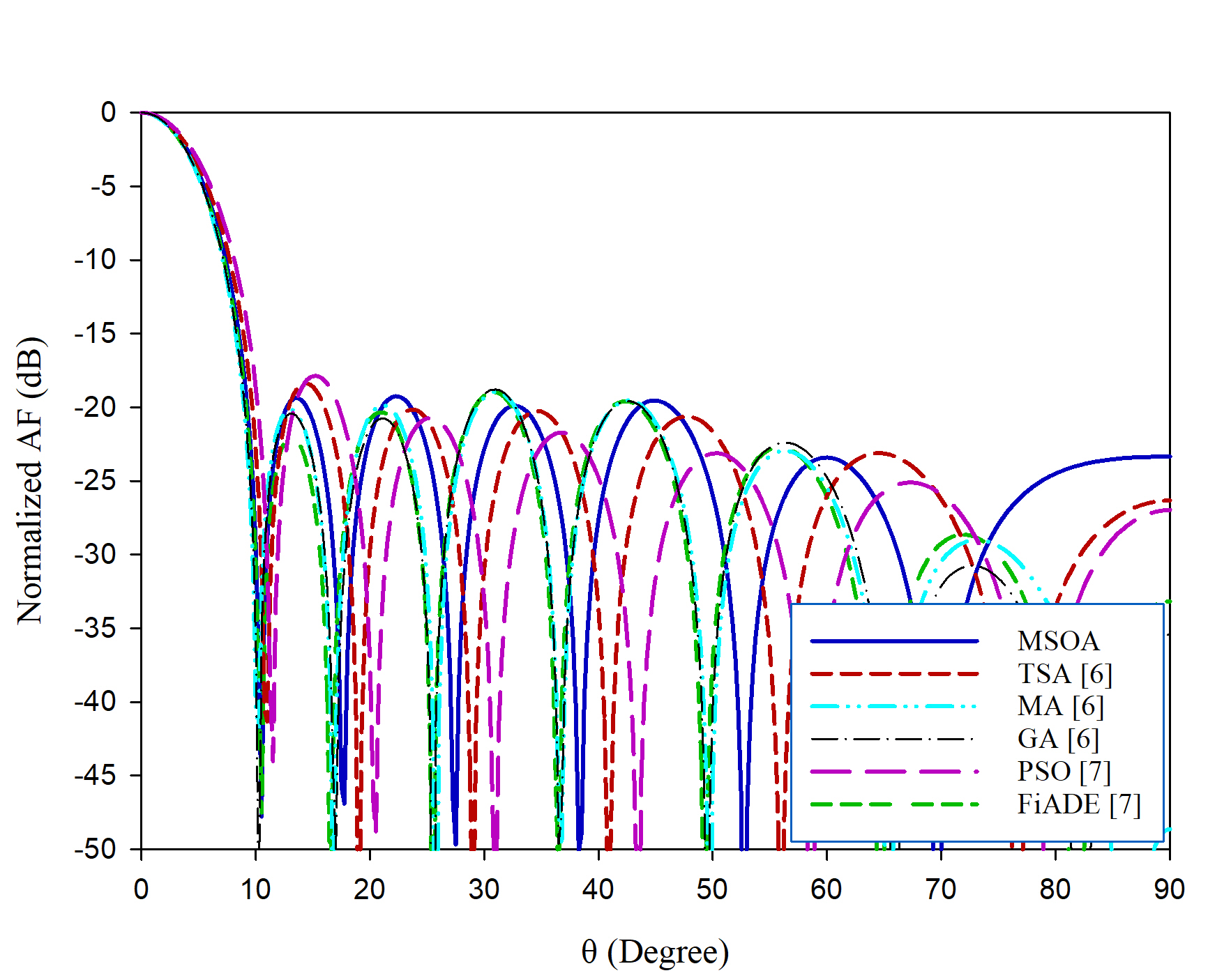
Figure 9: Radiation patterns optimized by MSOA and compared algorithms TSA [6], MA [6], GA [6], PSO [7], and FiADE [7] for 12-element LAA.
Table 5: Comparison of the MSL values for 12-element LAA design by controlling the positions of array elements
| Algorithm | MSOA | TSA [6] | MA [6] | GA [6] | PSO [7] | FiADE [7] |
| MSL (dB) | –19.25 | –18.40 | –19.10 | –18.77 | –17.90 | –18.96 |
Table 6: MSL and NDL values of the patterns achieved by MSOA and other optimization algorithms for 22-element LAA with null at 9
| Algorithm | MSOA | TSA [6] | MA [6] | PSO [7] | HSA [9] | BSA [10] |
|---|---|---|---|---|---|---|
| MSL (dB) | –23.90 | –17.17 | –18.11 | –20.68 | –23.28 | –23.54 |
| NDL (dB) (9) | –119.80 | –67.94 | –73.92 | –49.94 | –103.30 | –104.61 |
Table 7: NDL and MSL values of the patterns obtained by MSOA, BSA [10], CLPSO [11], and MVMO [12] for 28-element LAA with nulls at 30, 32.5, and 35
| Algorithm | MSOA | BSA [10] | CLPSO [11] | MVMO [12] |
| MSL (dB) | –22.57 | –21.90 | –21.63 | –21.63 |
| NDL (dB) (30) | –87.10 | –82.49 | –60.04 | –70.19 |
| NDL (dB) (32.5) | –103.30 | –93.59 | –60.01 | –78.79 |
| NDL (dB) (35) | –86.56 | –80.49 | –60.00 | –71.79 |
In the fifth example, the element positions of 2 N = 22 element LAA are optimized by means of MSOA to obtain a radiation pattern with nulls at 9 as well as the low MSL values. Figure 10 presents the radiation pattern calculated by MSOA. The figure also includes the radiation patterns produced by TSA [6], MA [6], PSO [7], HSA [9], and BSA [10]. Table 6 gives the MSL and NDL comparisons between MSOA and the other algorithms. From the table, it can be said that MSOA achieved better MSL and NDL values than the other algorithms.
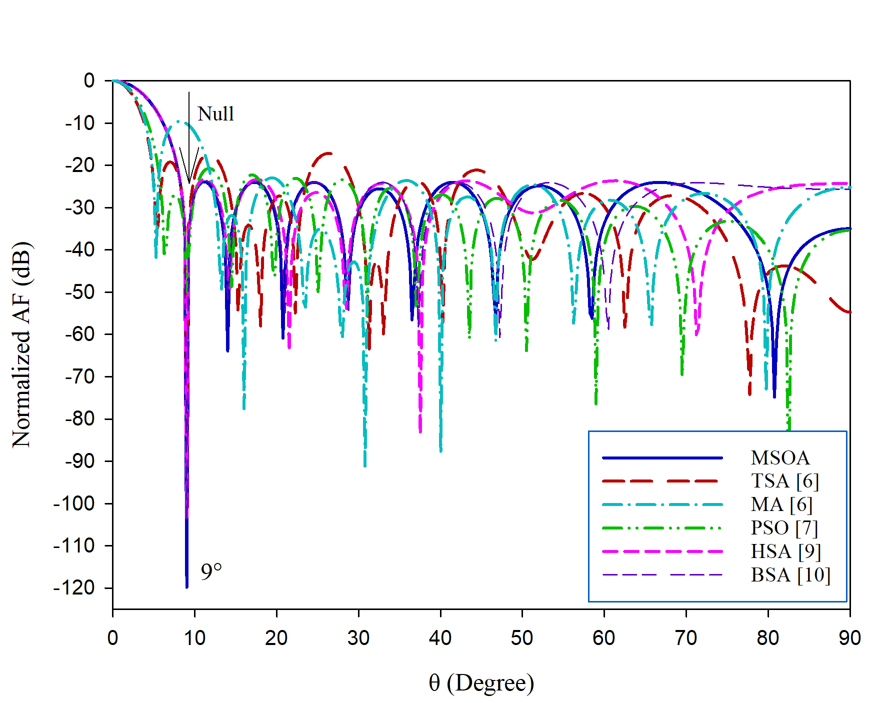
Figure 10: Radiation patterns with null at 9 optimized by MSOA and compared algorithms TSA [6], MA [6], PSO [7], HSA [9], and BSA [10] for 22-element LAA.
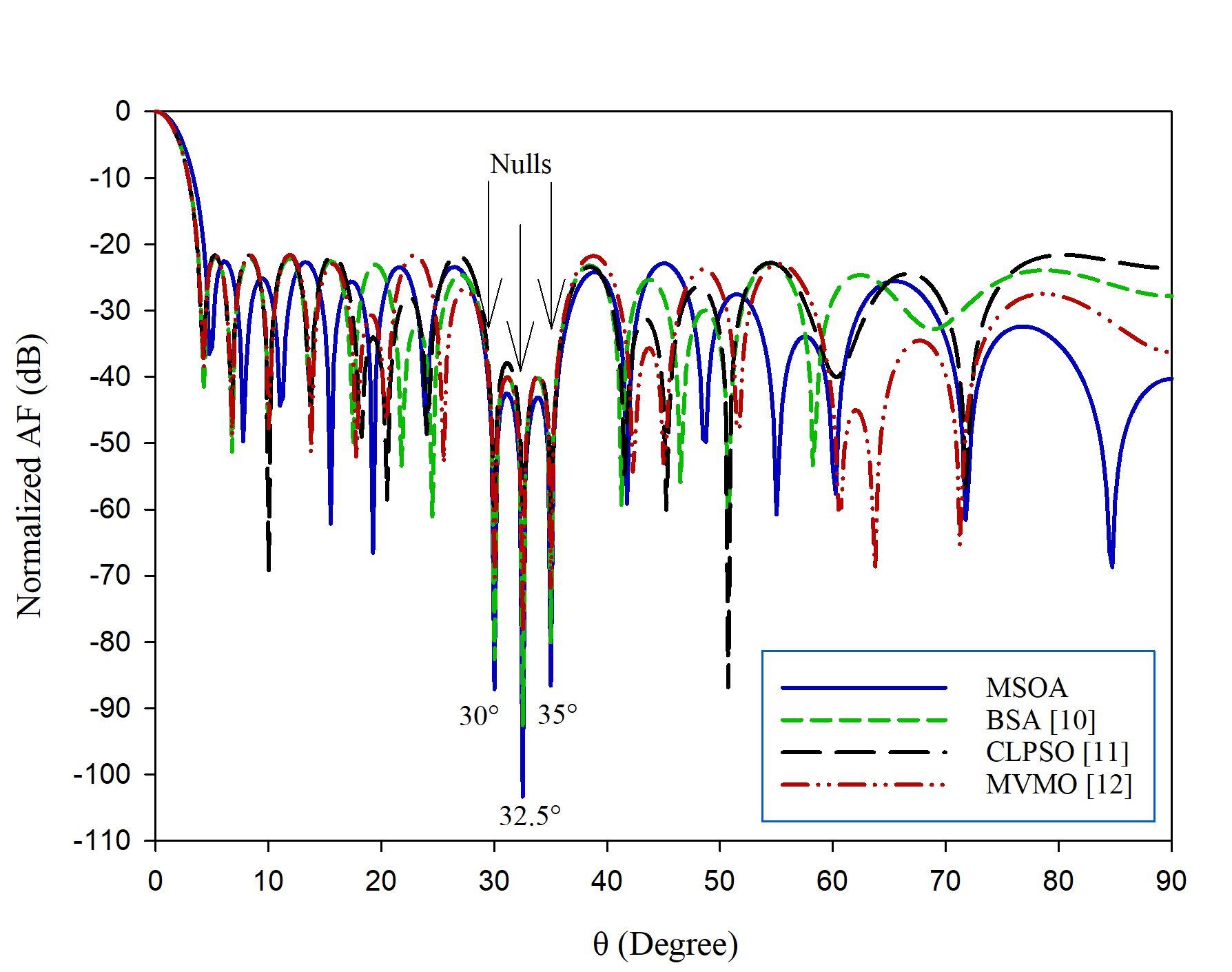
Figure 11: Radiation patterns with nulls at 30, 32.5, and 35 optimized by MSOA and compared algorithms BSA [10], CLPSO [11], and MVMO [12] for 28-element LAA.
There are two differences between the fifth and sixth examples. The first one is that the LAA considered in the sixth example is 2N = 28 element antenna array. As a second difference from the fifth example, in the sixth example, multiple nulls (30, 32.5, and 35) are placed on the radiation pattern instead of a single null. The resultant array pattern with a low MSL value and multiple nulls at 30, 32.5, and 35 is given in Figure 11. The figure also owns the array patterns obtained by BSA [10], CLPSO [11], and MVMO [12]. For a more precise comparison, The MSL and NDL values obtained by MSOA and the other algorithms are tabulated in Table 7. From Table 7, it can be concluded that MSOA has achieved better values than the other algorithms in terms of MSL and NDL parameters.
For the last example, the number of elements is increased to 2N = 32 to test MSOA for a larger parametric dimension. The target in this example is to achieve a pattern with a low MSL and a deep NDL at 9. Figure 12 presents the radiation patterns calculated by MSOA and the other algorithms including PSO [8], HSA [9], and BSA [10] from the literature. Table 8 gives the MSL and NDL values of the radiation patterns given in Figure 12. It is apparent from the figure and the table that MSOA has obtained better MSL and NDL results than the compared algorithms.
Table 8: Comparison of results of different algorithms for 32-element LAA with null at 9
| Algorithm | MSOA | PSO [8] | HSA [9] | BSA [10] |
|---|---|---|---|---|
| MSL (dB) | –21.49 | –18.80 | –19.51 | –20.50 |
| NDL (dB) (9) | –114.50 | –62.20 | –88.08 | –107.50 |
Table 9: Element positions optimized by MSOA for the array patterns given in Figures 9–12
| Number of elements | [d, d, …, d] |
|---|---|
| 12 (Figure 9) | [0.4206 1.2580 2.2039 3.1671 4.4298 5.7448] |
| 22 (Figure 10) | [0.2804 0.8094 1.3807 1.9663 2.4326 3.2601 3.7161 4.6507 5.3881 6.5371 7.6742] |
| 28 (Figure 11) | [0.5756 1.0542 2.1406 2.7600 3.7187 4.4164 5.3123 6.1621 7.3610 8.2936 9.3923 |
| 11.0114 12.5343 14.0927] | |
| 32 (Figure 12) | [0.2150 1.2795 1.9403 2.7564 3.2846 4.2449 5.0273 5.7899 6.4887 7.2680 8.1098 |
| 8.9617 10.4744 11.9414 13.7327 15.3084] |
The element position values calculated by the MSOA for the patterns given in Figures 9, 10, 11, 12 are tabulated in Table 9.
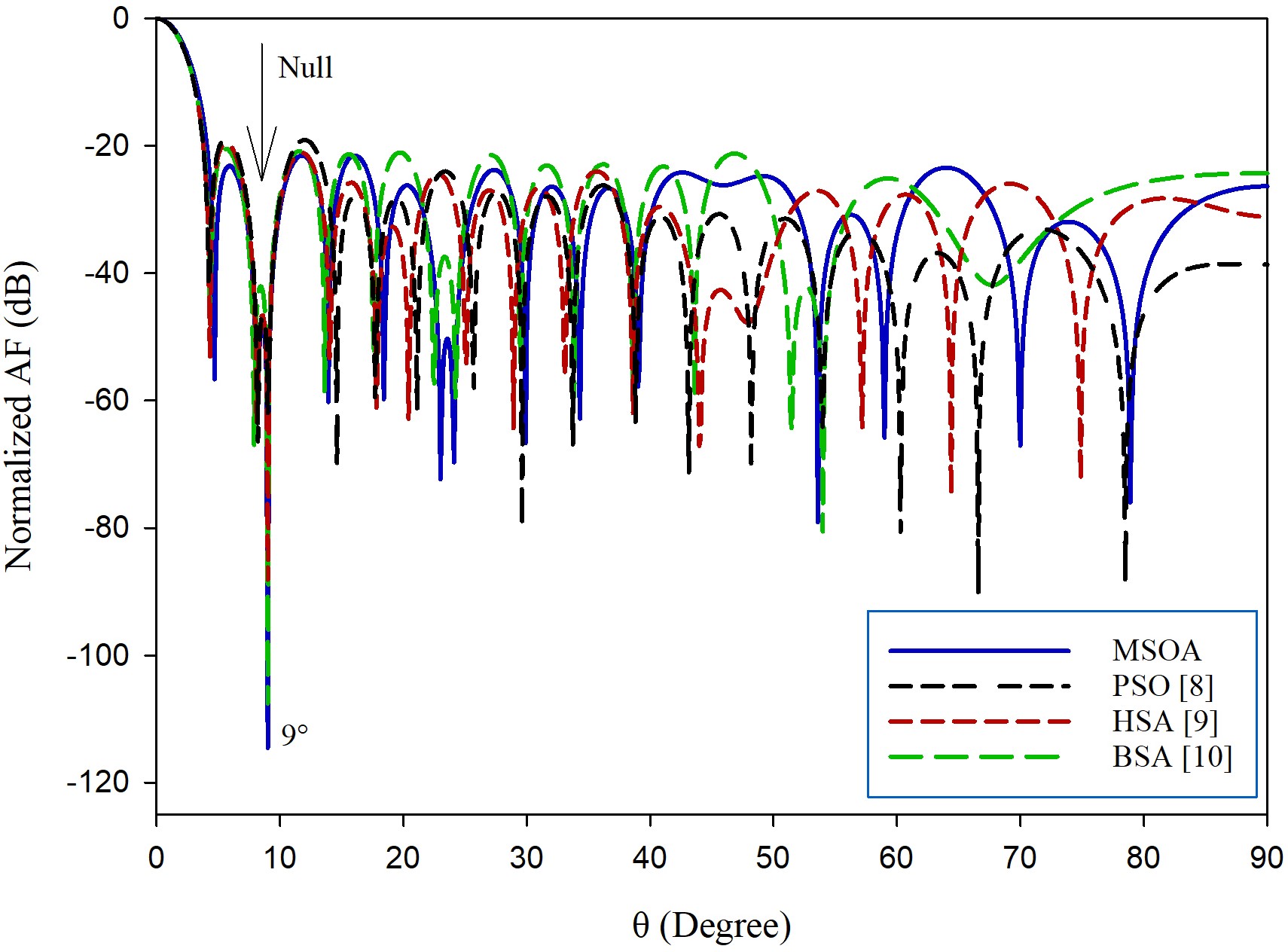
Figure 12: Radiation patterns with null at 9 optimized by MSOA and compared algorithms PSO [8], HSA [9], and BSA [10] for 32-element LAA.
V. CONCLUSION
In this paper, MSOA, a modified version of SOA, is employed to optimize the array amplitude and position values in order to achieve desired radiation patterns. Seven examples including 10-, 12-, 16-, 22-, 28-, and 32-elements LAA are considered for different purposes. The main idea in this work is to produce radiation patterns with low MSL and deep NDL values. From the overall results, it can be concluded that MSOA has a good performance to synthesize LAA radiation patterns.
It is also shown that the modification on SOA proposed in this article ensures that the algorithm converges faster. The comparisons with the other algorithms from the literature show that MSOA is a very good competitor in the engineering optimization field. Although MSOA is used for LAAs in this study, it can be apparently said that the algorithm is suitable to be used for the other array geometries such as circular, elliptical, and planar.
REFERENCES
[1] C. A. Balanis, Antenna Theory: Analysis and Design, vol. 1, John Wiley & Sons, 2005.
[2] P. Saxena and A. Kothari, “Optimal pattern synthesis of linear antenna array using grey wolf optimization algorithm,” International Journal of Antennas and Propagation, vol. 2016,2016.
[3] A. Das, D. Mandal, S. P. Ghoshal, and R. Kar, “Moth flame optimization based design of linear and circular antenna array for side lobe reduction,” International Journal of Numerical Modelling: Electronic Networks, Devices and Fields, vol. 32, no. 1, e2486, 2019.
[4] P. Saxena and A. Kothari, “Ant lion optimization algorithm to control side lobe level and null depths in linear antenna arrays,” AEU-International Journal of Electronics and Communications, vol. 70, no. 9, pp. 1339-1349, 2016.
[5] A. Sharaqa and N. Dib, “Design of linear and elliptical antenna arrays using biogeography based optimization,” Arabian Journal for Science and Engineering, vol. 39, pp. 2929-2939, 2014.
[6] Y. Cengiz and H. Tokat, “Linear antenna array design with use of genetic, memetic and tabu search optimization algorithms,” Progress in Electromagnetics Research C, vol. 1, pp. 63-72, 2008.
[7] A. Chowdhury, R. Giri, A. Ghosh, S. Das, A. Abraham, and V. Snasel, “Linear antenna array synthesis using fitness-adaptive differential evolution algorithm,” In IEEE Congress on Evolutionary Computation, IEEE, pp. 1-8, July 2010.
[8] M. M. Khodier and C. G. Christodoulou, “Linear array geometry synthesis with minimum sidelobe level and null control using particle swarm optimization,” IEEE Transactions on Antennas and Propagation, vol. 53, no. 8, pp. 2674-2679, 2005.
[9] K. Guney and M. Onay, “Optimal synthesis of linear antenna arrays using a harmony search algorithm,” Expert Systems with Applications, vol. 38, no. 12, pp. 15455-15462, 2011.
[10] K. Guney and A. Durmus, “Pattern nulling of linear antenna arrays using backtracking search optimization algorithm,” International Journal of Antennas and Propagation, vol. 2015, 2015.
[11] S. K. Goudos V. Moysiadou, T. Samaras, K. Siakavara, and J. N. Sahalos, “Application of a comprehensive learning particle swarm optimizer to unequally spaced linear array synthesis with sidelobe level suppression and null control,” IEEE Antennas and Wireless Propagation Letters, vol. 9, pp. 125-129, 2010.
[12] K. Guney and S. Basbug, “Linear antenna array synthesis using mean variance mapping method,” Electromagnetics, vol. 34, no. 2, pp. 67-84, 2014.
[13] K. Guney and S. Basbug, “Null synthesis of time-modulated circular antenna arrays using an improved differential evolution algorithm,” IEEE Antennas and Wireless Propagation Letters, vol. 12, pp. 817-820, 2013.
[14] A. Sharaqa and N. Dib, “Circular antenna array synthesis using firefly algorithm,” International Journal of RF and Microwave Computer-Aided Engineering, vol. 24, no. 2, pp. 139-146, 2014.
[15] A. E. Taser, K. Guney, and E. Kurt, “Circular antenna array synthesis using multiverse optimizer,” International Journal of Antennas and Propagation, vol. 2020, 2020.
[16] G. Ram, D. Mandal, R. Kar, and S. P. Ghoshal, “Circular and concentric circular antenna array synthesis using cat swarm optimization,” IETE Technical Review, vol. 32, no. 3, pp. 204-217, 2015.
[17] P. Civicioglu, “Circular antenna array design by using evolutionary search algorithms,” Progress in Electromagnetics Research B, vol. 54, pp. 265-284, 2013.
[18] A. S. Zare and S. Baghaiee, “Application of ant colony optimization algorithm to pattern synthesis of uniform circular antenna array,” Applied Computational Electromagnetics Society Journal, vol. 30, no. 8, pp. 810-818, 2015.
[19] N. Dib, A. Amaireh, and A. Al-Zoubi, “On the optimal synthesis of elliptical antenna arrays,” International Journal of Electronics, vol. 106, no. 1, pp. 121-133, 2019.
[20] A. A. Amaireh, N. Dib, and A. S. Al-Zoubi, “The optimal synthesis of concentric elliptical antenna arrays,” International Journal of Electronics, vol. 107, no. 3, pp. 461-479, 2020.
[21] V. V. S. S. S. Chakravarthy, P. S. R. Chowdary, N. Dib, and J. Anguera, “Elliptical antenna array synthesis using evolutionary computing tools,” Arabian Journal for Science and Engineering, pp. 1-18, 2021.
[22] A. Smida, R. Ghayoula, A. Ferchichi, A. Gharsallah, and D. Grenier, “Planar antenna array pattern synthesis using a taguchi optimization method,” International Journal on Communications Antenna and Propagation, vol. 3, no. 3, pp. 158–162, 2013.
[23] L. Zhang, Y. C. Jiao, B. Chen, and H. Li, “Orthogonal genetic algorithm for planar thinned array designs,” International Journal of Antennas and Propagation, vol. 2012, 2012.
[24] T. Sallam and M. A. Attiya, “Different array synthesis techniques for planar antenna array,” Applied Computational Electromagnetics Society Journal, vol. 34, no. 5, pp. 716-723, 2019.
[25] G. Dhiman and V. Kumar, “Seagull optimization algorithm: Theory and its applications for large-scale industrial engineering problems,” Knowledge-Based Systems, vol. 165, pp. 169-196, 2019.
[26] Y. Cao, Y. Li, G. Zhang, K. Jermsittiparsert, and N. Razmjooy, “Experimental modeling of PEM fuel cells using a new improved seagull optimization algorithm,” Energy Reports, vol. 5, pp. 1616-1625, 2019.
[27] H. Jiang, Y. Yang, W. Ping, and Y. Dong, “A Novel Hybrid Classification Method Based on the Opposition-Based Seagull Optimization Algorithm,” IEEE Access, vol. 8, pp. 100778-100790, 2020.
[28] G. Lei, H. Song, and D. Rodriguez, “Power generation cost minimization of the grid-connected hybrid renewable energy system through optimal sizing using the modified seagull optimization technique,” Energy Reports, vol. 6, pp. 3365-3376, 2020.
BIOGRAPHIES

Erhan Kurt was born in 1988. He received his M.Sc. from the Erciyes University in 2014. He is currently employed as a research assistant at Nuh Naci Yazgan University, Electrical and Electronics Engineering Department and working towards the Ph.D. degree in Electrical and Electronics Engineering at Erciyes University. His research interests include antennas and antenna arrays.

Suad Basbug received the B.S. and Ph.D. degrees in electrical and electronics engineering from Erciyes University, Kayseri, in 2008 and 2014, respectively. He has been an assistant professor at Nevsehir Haci Bektas Veli University since 2014. His current research interests include antennas, antenna arrays, conformal antennas, evolutionary algorithms, and computational electromagnetics.

Kerim Guney received the B.S. degree from Erciyes University, in 1983, the M.S. degree from Istanbul Technical University, in 1988, and the Ph.D. degree from Erciyes University, in 1991, all in electronics engineering. He is now a Professor in the Department of Electrical and Electronics Engineering, Nuh Naci Yazgan University. His research interests include antennas, planar transmission lines, optimization algorithms, and targettracking.
ACES JOURNAL, Vol. 36, No. 12, 1552–1562.
doi: 10.13052/2021.ACES.J.361206
© 2021 River Publishers