Modeling the Performance Impact of Anisotropic Unit Cells Used in Additively Manufactured Luneburg Lenses

Brian F. LaRocca${}^1$ and Mark S. Mirotznik${}^2$

¹Department of the Army,
Aberdeen Proving Ground, Aberdeen, MD 21005, USA
brian.f.larocca.civ@army.mil

²Electrical Engineering Department,
University of Delaware, Newark, DE 19716, USA
mirotzni@udel.edu

Submitted On: September 24, 2021; Accepted On: January 28, 2022

Abstract

Additively manufactured graded index lenses, such as the Luneburg lens, often result in some degree of uniaxial anisotropy in the effective permittivity distribution. A uniaxially anisotropic Luneburg lens modifies the polarization state of an incident electromagnetic field, thus giving rise to a polarization mismatch at the receiving antenna. Using 3D finite element simulation, the lens focal point polarization is analyzed and a model that fits the simulation data is created. The model allows prediction of polarization mismatch loss given any incident field and any receiving antenna polarization without resorting to further time-consumingsimulations.

Keywords: Anisotropic lens, finite element analysis, Luneburg lens, 3D printing.

I. INTRODUCTION

Numerous researchers have reported on the use of sub-wavelength unit cells as fundamental building blocks to additively manufacture graded index components such as the Luneburg lens [1–9]. In these accounts, a 3D printer dispenses precise amounts of material within each unit cell volume, thus controlling the effective permittivity of the cell. Depending upon the complexity of the design, certain fabrication techniques and cell geometries are best suited in terms of manufacturability. Figure 1 provides sketches of two successful unit cell geometries that have been implemented. In (a), the researchers employ a lattice of ultraviolet-curable polymer cubes with interconnecting rods [3], and, indeed, this design is isotropic. The implementation uses a polymer-jetting technique that requires an interposed water-soluble polymer that supports the lattice as it is being printed. This material must then be thoroughly flushed out of the part before use. For complex or large designs with small unit cells, this flushing process of removing support material may be problematic. Furthermore, the UV curable polymers used in polymer-jetting have significantly higher loss tangents than thermoplastics [10]. For large designs, this results in an appreciable reduction in radiation efficiency. In (b), the authors in [1, 2] overcome these difficulties by using a planar unit cell, which is printed from a filament of melted thermoplastic, in a process known as fused deposition modeling. This technique produces a cost-effective, low loss, and sturdy design, without the need for a support material. However, the planar unit cell is uniaxially anisotropic. This anisotropy has been recognized by the authors in [1, 2], but its impact on lens performance has yet to be investigated.

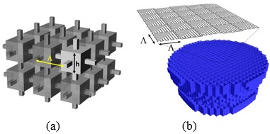
Figure 1: Unit cell geometries that have been created for 3D printing of graded index components. (a) UV-curable polymer cubes with interconnecting rods and (b) planer unit cell. A indicates the size of the unit cell, which is much smaller than the free-space wavelength at the intended operating frequency

Thus, this work uses 3D finite element simulations and post-processing to examine the performance impact of this unit cell anisotropy. A model is created to fit the field at the focal point, which then enables prediction of polarization state without further finite element simulation. The outline for the subsequent portion of the paper is as follows. Section II discusses the simulation environment, including an analysis of error. Section III provides the details of the anisotropy model that is incorporated into the simulations. Section IV develops the simplifying focal point model and Section V applies this model to predict polarization loss. Section VI then discusses the primary results.

II. SIMULATION ENVIRONMENT

The MATLAB partial differential equation (PDE) toolbox [11] is used to perform 3D finite element analysis of an anisotropic Luneburg lens illuminated by a monochromatic uniform plane wave. The toolbox is used to mesh the computational domain composed of the lens and free space and solve for the scattered field. Upon completion, the scattered field is summed with the incident field to obtain the total field solution [12].

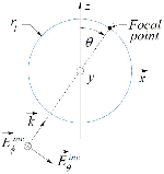
The computational domain is meshed using tetrahedral elements that have a maximum edge length of $l_{\max }\le 0.1\lambda$, where $\lambda$ is the free-space wavelength of the incident field. The computational domain is bounded by a sphere of radius $r_b=r_l+0.5\lambda$ that is concentric around the lens of radius $r_l$. A first-order absorbing boundary condition [12] is used over the bounding spheres surface. Due to the rotational symmetry of the lens about the $z$-axis, the direction vector $\overrightarrow{k}$ of the incident field is confined to the $x,z$ plane. The sketch in Figure 2 identifies the geometry of the simulation scenario excluding the outer spherical boundary, and a summary of simulation parameters is provided in Table 1.

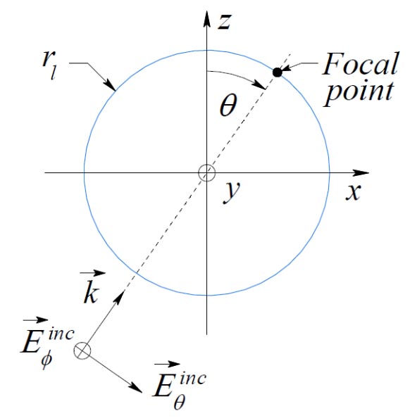
Figure 2: Incident plane wave, lens, and focal point.

Table 1: Simulation parameters

Category	Parameter	Value
Model	Frequency	15 GHz
	Plane wave polarization	Left hand circular
	Domain radius	$r_l+0.5\lambda$
Boundary conditions	First-order absorbing
Mesh	Max. edge length	$0.1\lambda$
	Nodes per element	4
	Growth rate	1.5
Solver	Type	lsqr()
	Tolerance	$0.1\times {10}^{-3}$
	Matrix conditioning	equilibrate()

Referring to the solver category in Table 1, lsqr() and equilibrate() are both core MATLAB functions designed to operate on sparse matrices. lsqr() implements the least squares method to solve the linear matrix equation $Ax=b$ for $x$. equilibrate(A) is used to the transform the linear system into an equivalent system that is very stable, prior to solution with lsqr(). Although the PDE toolbox provides solvepde() for this purpose, the underlying solveStationary() routine is not suitable for large problems, and in such cases, it is necessary to substitute an iterative solver such as gmres() or lsqr(). For the problems in this study, it was found that lsqr() performed the best. Another PDE toolbox function that is very useful is createPDEResults(). This utility function packs the solution $x$ into a structure that is identical to that returned by solvepde(). Drop-in compatibility is achieved by invoking this function before returning from a custom solver routine which may itself call either gmres() or lsqr().

Parameters $l_{\max }$ and $r_b$ have been chosen after experimentation, with the intent of striking a balance between solution fidelity and simulation efficiency. This experimentation includes evaluating isotropic reference lens simulations, which are shown in Table 2.

Table 2: Evaluation of simulation error with isotropic reference lens

$r_l$	$\mathrm{\angle }{E}_{\varphi }-\mathrm{\angle }{E}_{\theta }-{90}^{{}^{\circ }}$	$\left|E_{\varphi }\right|/\left|E_{\theta }\right|-1$
$2.5\lambda$	$+{3.37}^{{}^{\circ }}$	$+0.011$
$3.5\lambda$	$-{2.25}^{{}^{\circ }}$	$-0.017$
$5.0\lambda$	$-{1.21}^{{}^{\circ }}$	$+0.001$
RMS error	${2.44}^{{}^{\circ }}$	$0.012$

In this evaluation, three isotropic lenses of varying radii are illuminated with a left hand circularly polarized (LCP) plane wave. Given the incident field is LCP, the phase difference $\mathrm{\angle }{E}_{\varphi }-\mathrm{\angle }{E}_{\theta }$ at the focal point should precisely be equal to ${90}^{{}^{\circ }}$, and the polarization ratio $\left|E_{\varphi }\right|/\left|E_{\theta }\right|$ should precisely be equal to $1.0$. However, since $r_b<\mathrm{\infty }$ and $l_{\max }>0$, the observed root mean square (RMS) error is ${2.44}^{{}^{\circ }}$ in phase and 0.012 in polarization ratio.

A similar evaluation involves illuminating three uniaxially anisotropic lenses of varying radii, with an LCP plane wave at a polar angle of $\theta =0^{{}^{\circ }}$. The results of this test are shown in Table 3. Since the illumination is parallel to the optic axis of the lens, both $E_{\varphi }$ and $E_{\theta }$ experience equivalent material properties. Ideally then, the polarization state at the focal point should equal that of the incident wave, i.e., a $+{90}^{{}^{\circ }}$ phase difference with a polarization ratio of $1.0$ (just as in the isotropic case). The observed RMS error in this case is ${1.10}^{{}^{\circ }}$ in phase and 0.02 in polarization ratio. The observed errors in both the isotropic and anisotropic tests are deemed acceptable.

Table 3: Evaluation of simulation error with polar illumination of anisotropic lens

$r_l$	$\mathrm{\angle }{E}_{\varphi }-\mathrm{\angle }{E}_{\theta }-{90}^{\circ }$	$\left|E_{\varphi }\right|/\left|E_{\theta }\right|-1$
$2.5\lambda$	$-{0.43}^{\circ }$	$+0.013$
$3.5\lambda$	$+{0.94}^{\circ }$	$-0.018$
$5.0\lambda$	$+{1.60}^{\circ }$	$-0.026$
RMS error	${1.10}^{\circ }$	$0.020$

III. MODELING OF LENS ANISOTROPY

The model used herein follows the findings of researchers in [1, 2] who showed that because of the additive manufacturing process and choice of cell geometry, the lens exhibits a negative uniaxial anisotropy in which

${ϵ}_x={ϵ}_y={ϵ}_{xy}\ge {ϵ}_z.$

(1)

Moreover, the permittivities along the $x$- and $y$-axes of the lens follow the Luneburg profile exactly. That is, for any point within the lens at a radial distance $r$ from the lens center

${ϵ}_{xy}=2-{\left(\frac{r}{r_l}\right)}^2.$

(2)

The permittivity of the lens along the $z$-axis is modeled by the fractional mixing formula

${ϵ}_z={ϵ}_{xy}\left(1-\alpha \right)+\alpha {ϵ}_{\mathrm{MG}},$

(3)

where $\alpha$ is a parameter (the purpose of which is explained shortly) and ${ϵ}_{\mathrm{MG}}$ represents the effective relative permittivity determined by the Maxwell Garnett (MG) mixing rule for spherical inclusions embedded in a host medium [13]. For a host medium of free space, it is given by

${ϵ}_{\mathrm{MG}}=1+3f\frac{({ϵ}_i-1)}{{ϵ}_i+2-f({ϵ}_i-1)}.$

(4)

Here, ${ϵ}_i$ represents the relative permittivity of the inclusions, and $f$ represents the volume fill fraction of a unit cell, i.e., the volumetric ratio of material to free space within the cell. In the context of this work, ${ϵ}_i$ is the relative permittivity of the dielectric material used to print the lens, which is taken as pure thermoplastic with a ${ϵ}_i$ of $2.6$0. The authors in [1, 2] determined ${ϵ}_z$ for the exact unit cell geometry of Figure 1(b) using rigorous coupled wave analysis (RCWA). It is a testament to the scope of Equation (4) in that it generates results that closely match their analysis. It is also fortunate since the alternative is to model the structural geometry of the lens down to the unit cell. To do so accurately would require a mesh fine enough to accurately capture its smallest feature, that being the cell thickness of 0.12 mm [1]. Ultimately, this requires a mesh $l_{\max }$ 160 times smaller and a memory requirement on the order of ${160}^3$ times greater than that used for the present study. This is not feasible since for a lens with $r_l=2.5\lambda$, this amounts to a memory requirement of $2.2\times {160}^3$ gigabytes or equivalently $8.6$ petabytes.

Table 4 compares the MG mixing rule to the Bruggeman and coherent-potential mixing rules [13] in terms of fitting the RCWA predictions of ${ϵ}_z$ as reported in [1, 2]. The table provides the RMS difference between the respective mixing rule and those results. The MG mixing rule has the least RMS difference, thus providing the best fit.

Table 4: Comparison of mixing rules to RCWA

Mixing rule	RMS difference
Maxwell Garnett	$0.064$
Bruggeman	$0.098$
Coherent-potential	$0.109$

A linear relationship between $f$ and ${ϵ}_{xy}$ is assumed, such that

$f=\frac{({ϵ}_{xy}-1)}{({ϵ}_i-1)}.$

(5)

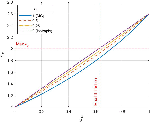
Finally, in Equation (3), the parameter $\alpha$ can range from 0 to 1 and is used to simulate designs that exhibit lesser degrees of anisotropy. For example, setting $\alpha$ equal $0$ generates a fully isotropic lens design since ${ϵ}_z={ϵ}_{xy}$, whereas setting $\alpha$ equal 1 generates the highest degree of anisotropy producing ${ϵ}_z={ϵ}_{MG}$. The MG equation with ${ϵ}_i=2.60$ is plotted in Figure 3 for four values of $\alpha$. The plot highlights the fact that for a chosen ${ϵ}_i$, the maximum fill fraction is $0.625$ which occurs at the lens center where ${ϵ}_z=2.0$.

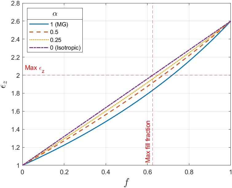
Figure 3: ${ϵ}_z$ vs. $f$ for different $\alpha$. Maximum ${ϵ}_z$ occurs at lens center where $f=0.625$.

IV. MODELING OF POLARIZATION

A. Illumination normal to optic axis

In this subsection, the lens is examined when it is illuminated with a plane wave normal to the $z$-axis of the lens. Referring to Figure 2, $\theta$ is therefore ${90}^{{}^{\circ }}$ and the incident field is simply directed along the $x$-axis of the lens. The incident field is represented as

${\overrightarrow{E}}^{\mathrm{inc}}=\left[\begin{array}{c}\hfill E_{\theta }^{\mathrm{inc}}\hfill \\ \hfill E_{\varphi }^{\mathrm{inc}}\hfill \end{array}\right]=\left[\begin{array}{c}\hfill a_{\theta }^{\mathrm{inc}}{e}^{j{\psi }_{\theta }^{\mathrm{inc}}}\hfill \\ \hfill a_{\varphi }^{\mathrm{inc}}{e}^{j{\psi }_{\varphi }^{\mathrm{inc}}}\hfill \end{array}\right]e^{-j{k}_{0}x},$

(6)

where $a_{\theta }^{\mathrm{inc}}\mathrm{and}{a}_{\varphi }^{\mathrm{inc}}$ are real positive constants, ${\psi }_{\theta }^{\mathrm{inc}}\mathrm{and}{\psi }_{\varphi }^{\mathrm{inc}}$ are real phase constants, and $k_0=2\pi /\lambda$. The illumination is LCP, where $a_{\theta }^{\mathrm{inc}}=a_{\varphi }^{\mathrm{inc}}$, and the phase difference ${\psi }_{\varphi }^{\mathrm{inc}}-{\psi }_{\theta }^{\mathrm{inc}}={90}^{{}^{\circ }}$. For a lens of radius $r_l$, the focal point is located on the surface of the lens, at the cartesian coordinate $(r_l,0,0)$. To assess the polarization at the focal point, the radial component of the resultant field at the focal point is ignored, leaving

$\overrightarrow{E}=\left[\begin{array}{c}\hfill a_{\theta }{e}^{j{\phi }_{\theta }}\hfill \\ \hfill a_{\varphi }{e}^{j{\phi }_{\varphi }}\hfill \end{array}\right],$

(7)

where $a_{\theta }\mathit{\hspace{1em}\hspace{1em} }\mathrm{and}{a}_{\varphi }$ are real positive values, and ${\phi }_{\theta }\mathit{\hspace{1em}\hspace{1em} }\mathrm{and}{\phi }_{\varphi }$are real phase terms and are different from the incident field constants in Equation (6). To describe the polarization state of the focal point, only the ratio $\sigma =a_{\varphi }/a_{\theta }$ and the phase difference $\delta ={\phi }_{\varphi }-{\phi }_{\theta }$ are required [15]. To create a simplifying polarization model of the lens that is independent of the incident field polarization state, the phase imbalance attributed to the lens itself is distinguished from $\delta$. We refer to this as the retardance of the lens $\acute{\delta }$, which is defined here as

$\acute{\delta }=\delta -({\psi }_{\varphi }^{\mathrm{inc}}-{\psi }_{\theta }^{\mathrm{inc}}).$

(8)

A similar distinction is required for the polarization ratio $\sigma$. Thus, we define the lens polarization ratio $\acute{\sigma }$ as being the polarization ratio measured at the focal point to ${\sigma }^{\mathrm{inc}}$, the polarization ratio of the incident field:

$\acute{\sigma }=\frac{\sigma }{{\sigma }^{\mathrm{inc}}}=\frac{a_{\varphi }/a_{\theta }}{a_{\varphi }^{\mathrm{inc}}/a_{\theta }^{\mathrm{inc}}}.$

(9)

Both $\acute{\sigma }$ and $\left|\acute{\delta }\right|$ take on maximum values when the illumination is normal to the optic axis. Under this condition, $\acute{\sigma }$ is referred to as ${\acute{\sigma }}_m$, and $\acute{\delta }$ is referred to as ${\acute{\delta }}_m$. Note that when the illumination is parallel, the optic axis $\acute{\sigma }=1$ and $\acute{\delta }=0$.

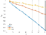
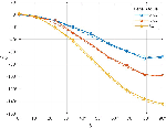
In the following two figures, the simulation results for $\acute{{\delta }_m}$ and ${\acute{\sigma }}_m$ are plotted using an $r_l$ from $0.5\lambda$to $6\lambda$, in $0.5\lambda$ increments. These results are shown for three values of the MG fractional anisotropy constant $\alpha$. This data is plotted with solid lines and markers. Additionally, polynomial least square fits to ${\acute{\delta }}_m$ and ${\acute{\sigma }}_m$ are plotted using dashed curves without markers; this data is comparatively smooth and sampled at a much finer resolution.

The least square fit for ${\acute{\delta }}_m$ is given by the first-order polynomial below and plotted with simulation data in Figure 4:

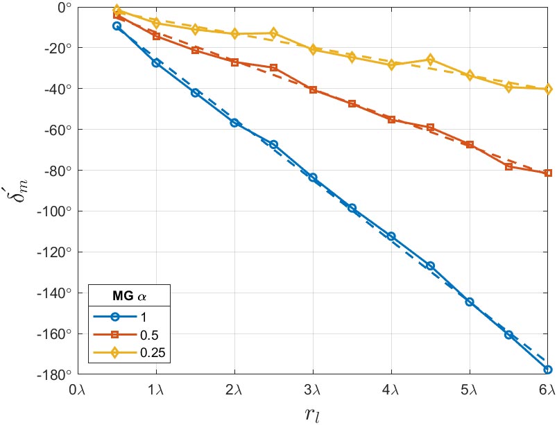
Figure 4: ${\acute{\delta }}_m$ vs. $r_l$ for different $\alpha$. Dashed lines are model given by least square fit in Equation (10).

${\acute{\delta }}_m=p_1\left[\alpha \right]{\overline{r}}_l+p_2\left[\alpha \right],$

(10)

where ${\acute{\delta }}_m$ is specified in radians, ${\overline{r}}_l=r_l/\lambda$ and is unitless, and $p_1$ and $p_2$ are real coefficients given in Table 5. Note that in Equation (10), the square brackets indicate that $\alpha$ is being treated as a lookup table index $-$ not a continuous variable.

Table 5: Polynomial coefficients for ${\acute{\delta }}_m$

$\alpha$	$p_1$	$p_2$
1.0	$-$0.5209	0.0828
0.5	$-$0.2433	0.0264
0.25	$-$0.1195	0.01118

${\acute{\sigma }}_m$ is treated as a function of ${\acute{\delta }}_m$, and, as can be inferred from Figure 4, ${\acute{\delta }}_m<0^{{}^{\circ }}$. Moreover, a piecewise model of ${\acute{\sigma }}_m$ is necessary, expressed herein as

${\acute{\sigma }}_m=\{\begin{array}{c}\hfill \begin{array}{cc}\hfill {\acute{\sigma }}_m^a,\hfill & \hfill \mathrm{if}-{180}^{{}^{\circ }}\le {\acute{\delta }}_m\hfill \end{array}\hfill \\ \hfill \begin{array}{cc}\hfill {\acute{\sigma }}_m^b,\hfill & \hfill \mathrm{otherwise}.\hspace{1em}\hspace{1em}\hspace{1em}\hspace{1em}\hspace{1em} \hfill \end{array}\hfill \end{array}$

(11)

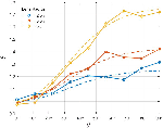
As ${\acute{\delta }}_m$ is varied from $0^{{}^{\circ }}$ to $-{180}^{{}^{\circ }}$, it is observed that $a_{\varphi }$ increases linearly, whereas $a_{\theta }$ increases non-linearly and settles into a plateau as ${\acute{\delta }}_m$ approaches $-{180}^{{}^{\circ }}$. For $-{180}^{{}^{\circ }}\le {\acute{\delta }}_m$, the least square fit for ${\acute{\sigma }}_m$ is given by the second-order polynomial below, and plotted with simulation data in Figure 5:

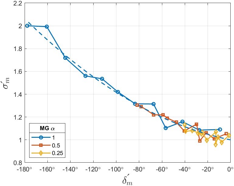
Figure 5: ${\acute{\sigma }}_m$ vs. ${\acute{\delta }}_m$ for different $\alpha$. Dashed curve is the model given by least square fit in Equation (12). For ${\acute{\delta }}_m<-{180}^{{}^{\circ }}$, the model transitions smoothly into the linear relationship given by Equation (13).

${\acute{\sigma }}_m^a=q_1{\acute{\delta }}_m^2+q_2{\acute{\delta }}_m+q_{3,}$

(12)

where $q_1$, $q_2$, and $q_3$ are the real coefficients given in Table 6.

Table 6: Polynomial coefficients for ${\acute{\sigma }}_m^a$

$q_1$	$q_2$	$q_3$
0.07122	$-$0.1148	0.9999

As ${\acute{\delta }}_m$ decreases beyond $-{180}^{{}^{\circ }}$, $a_{\varphi }$ continues to increase linearly, whereas $a_{\theta }$ is fixed at the plateau value. Therefore, ${\acute{\sigma }}_m$ is linear in this region and is given by

${\acute{\sigma }}_m^b=q_4{\acute{\delta }}_m+q_5,$

(13)

where the coefficients $q_4$ and $q_5$ are determined as follows. To ensure a differentiable, and thus continuous, piecewise model, the slope of the line defined by Equation (13) must equal the derivative of Equation (12) at ${\acute{\delta }}_m=-\pi$. Therefore

$q_4={\frac{d{\acute{\sigma }}_m^a}{d{\acute{\delta }}_m}|}_{{\acute{\delta }}_m=-\pi }=-2q_1\pi +q_2.$

(14)

Now, upon substituting Equation (14) into Equation (13), setting ${\acute{\sigma }}_m^b={\acute{\sigma }}_m^a$ and solving for $q_5$ at ${\acute{\delta }}_m=-\pi$ yields

$q_5={\left({\acute{\sigma }}_m^a-q_4{\acute{\delta }}_m\right)|}_{{\acute{\delta }}_m=-\pi }=q_3-q_1{\pi }^2.$

(15)

The piecewise model for ${\acute{\sigma }}_m$ therefore transitions smoothly between a second-order and a first-order polynomial at ${\acute{\delta }}_m={180}^{{}^{\circ }}$.

Equation (10) and (11), therefore, predict the extent to which the incident polarization state is altered when the incident wave is normal to the optic axis of thelens.

B. Illumination at arbitrary polar angle

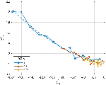
In this subsection, the impact of the lens anisotropy is examined as the polar angle $\theta$ of the incident field is swept from $0{}^{\circ }$ to ${90}^{{}^{\circ }}$ in ${11.25}^{{}^{\circ }}$ increments. The incident field is therefore defined as

${\overrightarrow{E}}^{\mathrm{inc}}=\left[\begin{array}{c}\hfill a_{\theta }^{\mathrm{inc}}{e}^{j{\psi }_{\theta }^{\mathrm{inc}}}\hfill \\ \hfill a_{\varphi }^{\mathrm{inc}}{e}^{j{\psi }_{\varphi }^{\mathrm{inc}}}\hfill \end{array}\right]e^{-j{k}_0\left(x\sin \left(\theta \right)+z\cos (\theta )\right)}.$

(16)

In this experiment, three different lens radii are studied: $2.5\lambda$, $3.5\lambda$, and $5\lambda$. It is observed that $\acute{\delta }=0$ when the incident field is parallel to the optic axis, i.e., $\theta =0^{{}^{\circ }}$, and $\acute{\delta }={\acute{\delta }}_m$ when the incident field is normal to it, i.e., $\theta ={\mathrm{\hspace{0.25em}90}}^{{}^{\circ }}$. Moreover, the retardance is approximatedby

$\acute{\delta }={\acute{\delta }}_m{\sin }^2\left(\theta \right).$

(17)

The retardance computed directly from the 3D finite element simulations and the approximation given in Equation (17) are plotted in Figure 6.

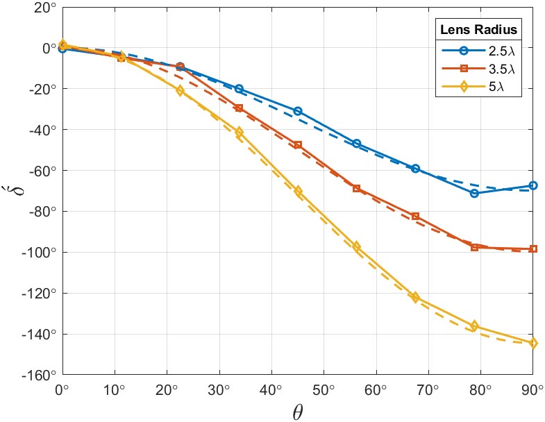
Figure 6: $\acute{\delta }$ vs. $\theta$ for different $r_l$. Dashed curves are model given by Equation (17).

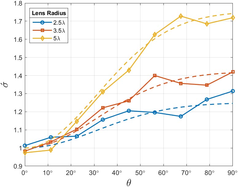
Figure 7: $\acute{\sigma }$ vs. $\theta$ for different $r_l$. Dashed curves are model given by Equation (18).

Correspondingly, $\acute{\sigma }=1$ when the incident field is parallel to the optic axis and $\acute{\sigma }={\acute{\sigma }}_m$ when the incident field is normal to it. After experimenting with several approximating functions, the following provides the best fit of $\acute{\sigma }$ to the simulation data:

$\acute{\sigma }=1+\frac{\left({\acute{\sigma }}_m-1\right)\left(1-e^{-{\left(\theta /\tau \right)}^2}\right)}{1-e^{-\left(\pi /2\tau \right)}{}^2}.$

(18)

In the above equation, $\theta$ is specified in radians and $\tau$ is a parameter that has been set to $0.6$ radians through experimentation. In Figure 7, both the results computed from the 3D finite element simulations and the approximation of Equation (18) are plotted.

Equation (17) and (18), therefore, predict the extent to which the incident polarization state is altered when the incident wave arrives at an arbitrary angle relative to the optic axis of the lens.

V. POLARIZATION LOSS

Other than for the degenerate cases in which either $a_{\theta }^{\mathrm{inc}}=0$ or $a_{\varphi }^{\mathrm{inc}}=0$, the anisotropy of the lens creates a mismatch between the incident and focal point polarizations. Normally, the receiving antenna has a polarization matched to that of the incident field. When the lens alters the incident polarization, the ability of the antenna to transfer focal power to the load is reduced. A non-dissipative loss is associated with this inefficiency and is termed the polarization loss factor (PLF). It is defined as follows [14]:

$\mathrm{PLF}=10\mathrm{l}\mathrm{o}{\mathrm{g}}_{10}\left(\mathrm{\Gamma }\right),$

(19)

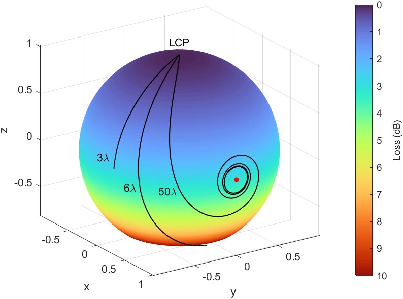
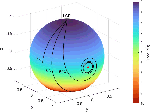
Figure 8: Paths on Poincarè sphere for different $r_l$, as $\theta$ is swept from $0^{\circ }$ to ${90}^{\circ }$. Surface of sphere indicates the PLF. Red dot is LHP marker. Illumination is LCP.

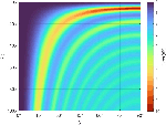
Finally, in Figure 9, the model provides PLF for a relatively wide range of lens radii with LCP illumination. The loss over most of the image is $\approx 3$ dB, indicating a focal point that is nearly horizontally polarized.

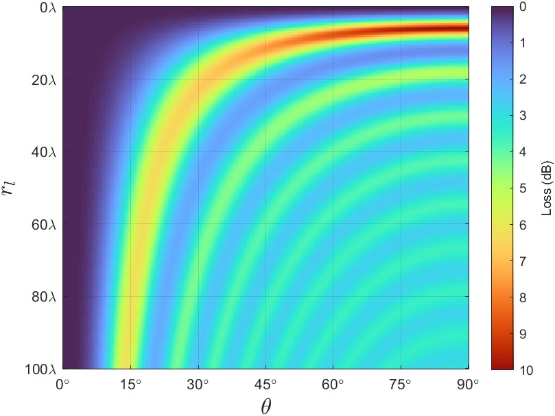
Figure 9: PLFs as $r_l$ and $\theta$ are varied. Compare with results on Poincarè sphere. Illumination is LCP.

where

$\mathrm{\Gamma }={\left|\widehat{\rho }\cdot {\widehat{\rho }}_r^{*}\right|}^2={\left|\cos \left({\psi }_r\right)\right|}^2.$

(20)

In Equation (20), $\widehat{\rho }$ is the unit polarization vector of the field at the focal point, ${\widehat{\rho }}_r^{*}$ is the complex conjugate of the unit polarization vector for the receiving antenna, and ${\psi }_r$ is the angle between the two. Since Equation (7) can be expressed as

$\overrightarrow{E}=a_{\theta }{e}^{j{\phi }_{\theta }}\left[\begin{array}{c}\hfill 1\hfill \\ \hfill \sigma e^{j\delta }\hfill \end{array}\right],$

(21)

then the direction of $\overrightarrow{E}$, and therefore $\widehat{\rho }$, must depend only on $\sigma$ and $\delta$. Thus

$\widehat{\rho }=\frac{1}{\sqrt{1+{\sigma }^2}}\left[\begin{array}{c}\hfill 1\hfill \\ \hfill \sigma e^{j\delta }\hfill \end{array}\right].$

(22)

To compute the PLF using the focal point polarization model developed in the previous section, we first use Equation (17) to compute $\acute{\delta }$ and Equation (18) to compute $\acute{\sigma }$. Both values are independent of the incident field’s polarization; therefore, we use Equation (8) to solve for $\delta$ and Equation (9) to solve for $\sigma$. In other words

$\delta =\acute{\delta }+\left({\psi }_{\varphi }^{\mathrm{inc}}-{\psi }_{\theta }^{\mathrm{inc}}\right),$

(23)

and

$\sigma =\acute{\sigma }{\sigma }^{\mathrm{inc}}.$

(24)

An insight into the dependence of the PLF on $r_l$ and $\theta$ is obtained by tracing the focal point polarization state on a Poincarè sphere that is PLF colorized according to the incident field. This is accomplished efficiently using the model developed in the previous section along with Equation (19), (23), and (24). Figure 8 provides such results for lens radii of $3\lambda$, $6\lambda$, and $50\lambda$, all illuminated with LCP. For each lens, as $\theta$ is swept from $0^{{}^{\circ }}$ to ${90}^{{}^{\circ }}$, the state moves away from the zero loss LCP state. A maximum loss of $\approx 10$ dB is observed when $r_l=6\lambda$. For $r_l=50\lambda$, the maximum loss drops to $\approx 6$ dB, and the state follows a spiraling path toward the linear horizontally polarized (LHP) state, denoted as a red dot. Larger lenses produce even tighter spirals around the LHP state and incur a maximum loss that asymptotically approaches $3$ dB.

VI. CONCLUSION

A uniaxially anisotropic Luneburg lens modifies the polarization state of an incident wave, thus introducing a polarization mismatch loss at the focal point. This mismatch is dependent upon the wave polarization, the degree of anisotropy, the radius of the lens, and the wave angle of arrival. For $r_l\gg \lambda$, the anisotropy strongly polarizes the focal point along the horizontal plane. This mismatch is undesirable in most circumstances, and minimizing it requires prediction of the unit cell permittivities along the $x$-, $y$- and $z$-axes.

We show that curve fitting of 3D finite element simulations provides an efficient method to model the retardance and polarization ratio of the lens. This model and knowledge of the incident wave and receiving antenna polarizations are sufficient to predict the amount of polarization mismatch loss, enabling the selection of isotropic unit cell geometries that are suitable for fused deposition modeling.

REFERENCES

[1] Z. Larimore, S. Jensen, A. Good, J. Suarez and M. S. Mirotznik, “Additive manufacturing of Luneburg lens antennas using space filling curves and fused filament fabrication,” IEEE Transactions on Antennas and Propagation, vol. 66, no. 6, pp. 2818-2827, June 2018.

[2] S. Biswas, A. Lu, Z. Larimore, P. Parsons, A. Good, N. Hudak, B. Garrett, J. Suarez and M. S. Mirotznik, “Realization of modified Luneburg lens antenna using quasi-conformal transformation optics and additive manufacturing,” Microwave and Optical Technology Letters, vol. 61, no. 4, pp. 1022-1029, 2019.

[3] M. Liang, W. R. Ng, K. Chang, K. Gbele, M. E. Gehm, and H. Xin, “A 3-D Luneburg lens antenna fabricated by polymer jetting rapid prototyping,” IEEE Transactions on Antennas and Propagation, vol. 62, no. 4, pp. 1799-1807, April 2014.

[4] Y. Li, L. Ge, M. Chen, Z. Zhang, Z. Li, and J. Wang, “Multibeam 3-D-Printed Luneburg lens fed by magnetoelectric dipole antennas for millimeter-wave MIMO applications,” IEEE Transactions on Antennas and Propagation, vol. 67, no. 4, pp. 2923-2933, May 2019.

[5] S. Lei, K. Han, X. Li, and G. Wei, “A design of broadband 3-D-Printed circularly polarized spherical Luneburg lens antenna for X-Band,” IEEE Antennas and Wireless Propagation Letters, vol. 20, no. 4, April 2021.

[6] C. Wang, J. Wu, and Y. Guo, “A 3-D-Printed wideband circularly polarized parallel-plate Luneburg lens antenna,” IEEE Transactions on Antennas and Propagation, vol. 68, no. 6, June 2020.

[7] J. Chen, H. Chu, Y. Zhang, Y. Lai, M. Chen, and D. Fang, “Modified Luneburg lens for achromatic sub-diffraction focusing and directional emission,” IEEE Transactions on Antennas and Propagation, vol. 69, no. 11, November 2021.

[8] M. Yin, X. Y. Tian, L. L. Wu, and D. C. Li, “All-dielectric three-dimensional broadband Eaton lens with large refractive index range,” Applied Physics Letters 104, 094101 (2014).

[9] C. Babayi$\breve{g}$it, A. S. Evren, E. Bor, H. Kurt, and M. Turduev, “Analytical, numerical, and experimental investigation of a Luneburg lens system for directional cloaking,” Physical Review, vol. 99, iss. 4, April 2019.

[10] P. I. Deffenbaugh, R. C. Rumpf, K. H. Church, “Broadband microwave frequency characterization of 3-D printed materials,” IEEE Transactions on Components, Packaging and Manufacturing Technology, vol. 3, no. 12, pp. 2147-2155, December 2013.

[11] MATLAB, ver. 2021a, The Mathworks Inc., Natick, Massachusetts, 2021.

[12] J. M. Jin, D. Riley. Finite Element Analysis Of Antennas And Arrays. John Wiley & Sons Inc., New Jersey, 2009.

[13] A. Sihvola, Electromagnetic Mixing Formulas And Applications, The Institution of Engineering and Technology, London, 2008.

[14] C. A. Balanis, Antenna Theory - Analysis And Design, John Wiley & Sons Inc., New Jersey, 2005

[15] F. T. Ulaby, U. Ravaioli, Fundamentals Of Applied Electromagnetics, Pearson, 2015.

BIOGRAPHIES

Brian F. LaRocca received the B.S.E.E. and M.S.E.E. degrees from the New Jersey Institute of Technology, Newark, NJ, USA in 1985 and 2000 respectively. He is currently working toward the Ph.D. degree in electrical engineering with the University of Delaware, Newark, DE, USA.

From 1985 to 1996, he worked in industry, from 1996 to 2004 as a government contractor, and from 2004 to present as a civilian engineer with the Department of the Army, Ft. Monmouth, NJ, USA and Aberdeen Proving Ground, MD, USA.

Mark S. Mirotznik (Senior Member, IEEE) received the B.S.E.E. degree from Bradley University, Peoria, IL, USA, in 1988, and the M.S.E.E. and the Ph.D. degrees from the University of Pennsylvania, Philadelphia, PA, USA, in 1991 and 1992, respectively.

From 1992 to 2009, he was a Faculty Member with the Department of Electrical Engineering,The Catholic University of America, Washington, DC, USA. Since 2009, he has been a Professor and an Associate Chair for Undergraduate Programs with the Department of Electrical and Computer Engineering, University of Delaware, Newark, DE, USA. He holds the position of Senior Research Engineer with the Naval Surface Warfare Center, Carderock Division. His current research interests include applied electromagnetics and photonics, computational electromagnetics, multifunctional engineered materials, and additive manufacturing.

ACES JOURNAL, Vol. 37, No. 1, 50–57.
doi: 10.13052/2022.ACES.J.370106
© 2021 River Publishers

Abstract

I. INTRODUCTION

II. SIMULATION ENVIRONMENT

III. MODELING OF LENS ANISOTROPY

IV. MODELING OF POLARIZATION

A. Illumination normal to optic axis

B. Illumination at arbitrary polar angle

V. POLARIZATION LOSS

VI. CONCLUSION

REFERENCES

BIOGRAPHIES