Rule for Mode Coupling Efficiency in Optical Waveguide Crossing

Billel Bentouhami${}^{\mathbf{\text{1,2}}}$ and Zaia Derrar Kaddour${}^{\mathbf{\text{2}}}$

¹Universit$\acute{\mathrm{e}}$ Mohamed El Bachir El Ibrahimi de Bordj Bou Arreridj, Facult$\acute{\mathrm{e}}$ des Sciences et de la Technologie,
El-Anasser 34030, Algeria
billelbentouhami@gmail.com

²Universit$\acute{\mathrm{e}}$ des Sciences et de la Technologie Houari Boumedi`ne, Facult$\acute{\mathrm{e}}$ de Physique, Laboratoire d’Electronique
Quantique, BP 32 EL Alia 16111, Bab Ezzouar, Algiers, 16311, Algeria
kaddourz@yahoo.com

Submitted On: September 25, 2021; Accepted On: May 24, 2022

Abstract

Crossing an optical waveguide requires a beam coupling from free space to waveguide at the entrance plane and another beam coupling from waveguide to free space at the exit plane of the waveguide. The aim of this paper is to provide a simple rule expressing the relationship between the involved numbers of free and guided modes that efficiently rebuild the field at each end of the waveguide. Using a numerical program built on Maple software, the rule was determined to be effective independently of the ratio between the beam spot size and the waveguide radius.

Index Terms: Electromagnetic field, mode coupling, optical waveguide.

I. INTRODUCTION

Hollow dielectric optical waveguides are widely used in optical systems such as resonators [1, 2], optical transmission and communication systems [3], circular waveguide filters [4], and, nowadays, in integrated optics [5].

Many authors have described light propagation in cylindrical optical waveguides [6–9]. Transverse modes inside a waveguide can be divided into three families: transverse electric (TE), transverse magnetic (TM), and hybrid (EH) modes. Each family constitutes a complete and orthogonal set for expressing the radially symmetric electromagnetic field in the waveguide.

Apart from the propagation inside the waveguide, two check points need to be considered when crossing a waveguide which are its entrance and exit ports. At the entrance port, mode coupling occurs from free space to confined one and vice versa at the exit port. For both ends of the waveguide, mode coupling has been studied by considering the ratio between the beam spot size w and the radius of the waveguide a [10–13].

At the waveguide entrance plane, Smith [10] described earliest experiments performed by matching the fundamental mode from a conventional He–Ne laser into a hollow dielectric waveguide. The incident beam was focused in such a way that the beam waist w${}_{\mathrm{0}}$ occurred at the entrance plane of the dielectric waveguide. It is worth noting that Smith performed transmission measurement by matching the fundamental free mode into the fundamental guided mode. For a good matching, he experimentally found a ratio w${}_{\mathrm{0}}$/a = 0.49 which was however considerably different from the theoretical ratio w${}_{\mathrm{0}}$/a = 0.728 he considered.

Always for the entrance plane and as a function of w/a, Roullard and Bas [11] gave the fraction of the coupled energy from the free fundamental Gaussian mode TEM${}_{00}$ into the two first waveguide modes. They mentioned that an efficient coupling happens at w/a = 0.502. This value is different from the value w/a = 0.6435 that maximizes coupling with only the first-order waveguide mode as given by Abrams and Chester [12] and Tack [13].

At the waveguide exit plane, the useful approach to release mode coupling is founded on the use of a small number of free space modes but with a choice of a specific ratio w/a. Indeed, as mentioned by Guerlach [14], to minimize the truncation error in expanding the field emerging from the waveguide, a small value of the ratio is favored. But a small w results in a large divergence of the beam field and consequently a large truncation error. Avoiding this constraint of the w/a ratio choice requires a considerable number of modes with numerical problem consequences.

To conclude, either at the entrance or at the exit plane of the waveguide, mode coupling using a reduced number of modes is conditioned by the choice of the appropriate ratio w/a. Working with an arbitrary ratio, requires a large number of modes that unfortunately leads to numerical problems. Therefore, the question that we ask here is about the optimum number of modes that we should consider for realizing an efficient mode coupling regardless of a specific ratio w/a. To reach this goal, a simple rule is then given in this paper.

II. THEORY AND NUMERICAL RESULTS

Let us consider a hollow dielectric waveguide with a circular cross section of radius a, a length L, and a complex refractive index $\nu$. Assume that an incident beam is coming in from the left side as shown in Figure 1.

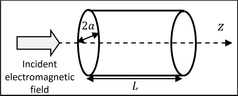
Figure 1: Incident beam to a cylindrical optical waveguide.

Crossing an optical waveguide is carried out in three successive steps which are: mode coupling at the entrance plane, propagating the derived guided electromagnetic field along the length L inside the waveguide, and finally performing mode coupling again at the exit plane to go back to free space. Figure 2 shows the sequence of operations undertaken in the waveguide crossing. This process requires normalized functions for free space and waveguide modes to be given.

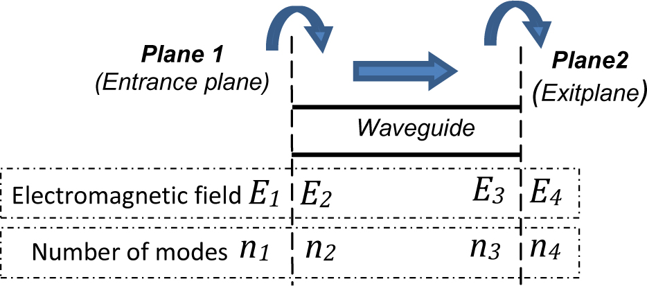
Figure 2: Sequence of operations undertaken in waveguide crossing.

In free space for the case of cylindrical symmetry, the normalized Laguerre Gauss functions are given by [15]

	${\mathrm{TEM}}_{pl}$
	$=\left({\displaystyle \frac{2}{w\sqrt{1+{\delta }_{0l}}}}\sqrt{{\displaystyle \frac{m!}{\pi \left(l+m\right)!}}}\right){\left({\displaystyle \frac{r}{w}}\sqrt{2}\right)}^l{L}_m^l\left(2{\displaystyle \frac{r^2}{w^2}}\right)$
	$\times \exp \left\{-{\displaystyle \frac{r^2}{w^2}}-j{\displaystyle \frac{k{r}^2}{2R}}\right\}\{\begin{array}{c}\hfill \cos \left(l\phi \right)\hfill \\ \hfill \sin \left(l\phi \right)\hfill \end{array},$	(1)

where r, $\phi$ are the cylindrical coordinates, $L_m^l$ is the generalized Laguerre polynomials, $\delta$ is the Kronecker symbol, j is the complex number such as $j^2=-1,$ and k is the wave number; R and w are the phase front radius and the spot size, respectively.

For the waveguide, the normalized hybrid functions with circular symmetry field are [14, 16]

$${\mathrm{EH}}_{1n}\left(r\right)=\{\begin{array}{cc}\begin{array}{cc}\hfill \frac{1}{\sqrt{\pi |J_1(u_{1n})|a}}{J}_0(\frac{u_{1n}r}{a})\hfill & \hfill r\le a\hfill \\ \hfill 0\hfill & \hfill r>a\hfill \end{array}\hfill & \end{array},$$

(2)

where $J_0$ and $J_1$ are the Bessel functions and $u_{1n}$is the nth root of the former one.

Mode coupling at each end of the waveguide is expressed using coupling coefficients$C_{\mathrm{mn}}$. These coefficients are reached by equalizing the electromagnetic fields at both sides of the considered waveguide port and they are given by [14]

$$C_{mn}=2\pi {\int }_0^{a}r{\mathrm{TEM}}_m\left(r\right){\mathrm{HE}}_n\left(r\right)\mathit{d}r.$$

(3)

As shown in Figure 2, mode coupling occurs at plane 1 using a number of excited guided modes $n_2$ and at plane 2 using a number of excited free space modes$n_4$. Simple rules giving the optimum $n_2$ and $n_4$ numbers for an efficient mode coupling are then the subject of Sections II-A and II-C.

A Rule for mode coupling at the waveguide entrance plane

The field equality $E_1=E_2$ inside the waveguide opening, at the entrance plane, is required for an efficient mode coupling. At both sides of this plane, the electromagnetic field is

$$E_1\left(r\right)=\sum _{m=1}^{n_1}{a}_m{\mathrm{TEM}}_m(r),$$

(4)

for the free space and

$$E_2\left(r\right)=\sum _{n=1}^{n_2}{C}_n{\mathrm{EH}}_n(r),$$

(5)

for the waveguide.

The integers $n_1$ and $n_2$ are the number of free space and waveguide modes, respectively; $a_{\mathrm{m}}$ represents the expansion coefficients of the incoming free field, whereas $C_{\mathrm{n}}$ are the derived expansion coefficients of the calculated guided field using eqn (3):

$$C_n=2\pi \sum _{m=1}^{n_1}{a}_m{C}_{mn}.$$

(6)

Table 1 gives, for each given number ${\mathit{\text{n}}}_{\mathbf{1}}$ of the used free space modes, the optimum number $n_2$ of waveguide modes which allows an efficient mode coupling at the waveguide entrance plane. This result is achieved for different w/a ratios.

Table 1: Optimized number $n_2$ of waveguide modes as a function of the number $n_1$ of the used free space modes

${\mathbf{n}}_{\mathbf{1}}$	${\mathbf{n}}_{\mathbf{2}}$
3	7
8	8
11	9
15	9
19	10
25	12
38	13
45	15
60	17
80	19
100	21

The plot $n_2$ versus $n_1$ is illustrated by the point curve in Figure 3.

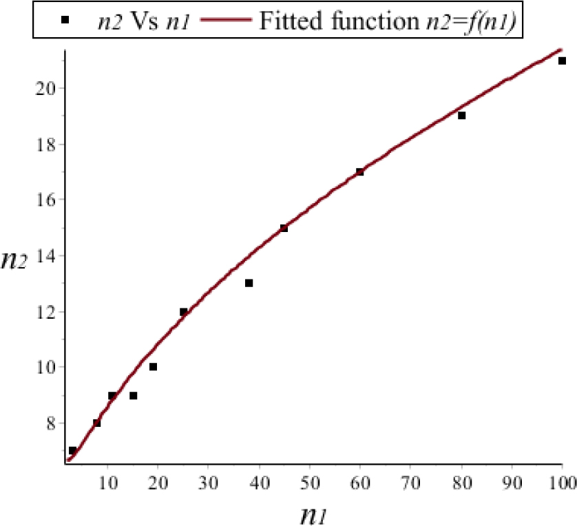
Figure 3: Optimized number $n_2$ of waveguide modes as a function of the number $n_1$ of the used free space modes.

Applying the mathematical fit instructions of Maple software using the data from Table 1, the appropriate function $n_2=f\left(n_1\right)$, shown in solid line in Figure 3, is deduced and the following rule for mode coupling at the waveguide entrance plane is obtained:

$$n_2=\lfloor 2\left(\sqrt{n_1}+\frac{2}{\sqrt{n_1}}\right)+1\rfloor ,$$

(7)

where the notation $\lfloor \mathrm{\square }\rfloor$ is the floor function.

For different $n_1$ and according to this rule, Figure 4 shows a very good agreement in field superposition for mode coupling at the entrance plane of thewaveguide.

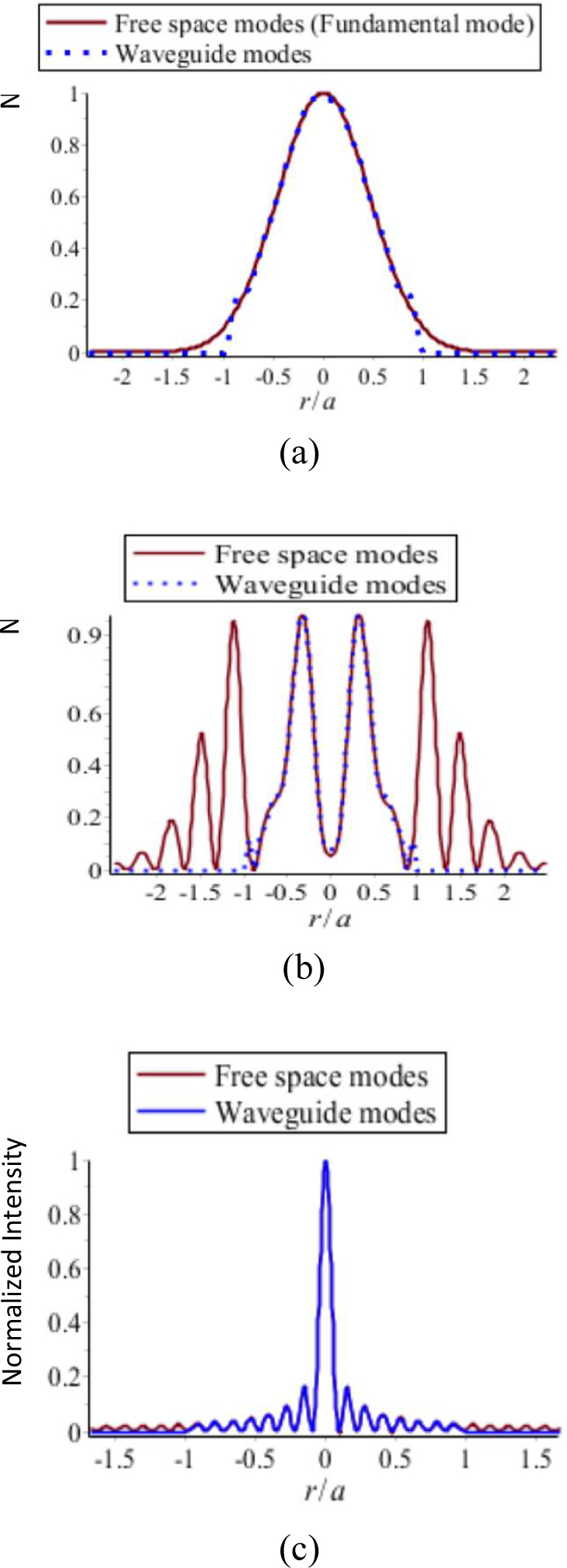
Figure 4: Superposition of transverse intensity patterns at the waveguide entrance plane with a = 0.6 mm for (a) $n_1$ = 1, (b) $n_1$ = 13, and (c) $n_1$ = 35.

The results shown in Figure 4 (a)–(c) have been computed with w/a = 0.91, w/a = 0.8, and w/a = 0.66, respectively. But we emphasize that for each case, and thanks to the rule, an efficient mode coupling has been confirmed for other arbitrary ratios w/a.

B Propagation inside the waveguide

Attenuation and relative phase shift of the propagating field, over a distance l through the waveguide, are calculated by multiplying each guided mode by the corresponding element of the following diagonalmatrix [14]:

	${\mathit{\text{CG}}}_{\mathit{\text{mn}}}={\delta }_{\mathit{\text{mn}}}\exp \left[{\mathit{\text{u}}}_{1\mathit{\text{m}}}^2\left({\displaystyle \frac{\mathit{\text{l}}}{{\mathit{\text{k}}\mathit{\text{a}}}^2}}\right)\mathrm{Re}\left({\displaystyle \frac{{\mathit{\text{v}}}_{\mathit{\text{n}}}}{\mathit{\text{ka}}}}\right)\right]$
	$\times \exp \left[-{\displaystyle \frac{\mathit{\text{i}}}{2}}\left({\mathit{\text{u}}}_{1\mathit{\text{m}}}^2-{\mathit{\text{u}}}_{11}^2\right)\left({\displaystyle \frac{\mathit{\text{l}}}{{\mathit{\text{k}}\mathit{\text{a}}}^2}}\right)\left(1+2\mathrm{Im}\left({\displaystyle \frac{{\mathit{\text{v}}}_{\mathit{\text{n}}}}{\mathit{\text{ka}}}}\right)\right)\right],$	(8)

where ${\delta }_{\mathit{\text{mn}}}$ is the Kronecker symbol, $\mathit{\text{k}}=2\pi /\lambda$, ${\mathit{\text{u}}}_{1\mathit{\text{m}}}$ is the mth zero of ${\mathit{\text{J}}}_0$ and ${\mathit{\text{v}}}_{\mathit{\text{n}}}=[{\mathit{\text{v}}}^2+1]/2{\left[{\mathit{\text{v}}}^2-1\right]}^{\frac{1}{2}}$ where $\nu$ is the complex refractive index of the waveguidematerial.

Figure 5 shows the electrical field intensity in different positions inside a cylindrical optical waveguide.

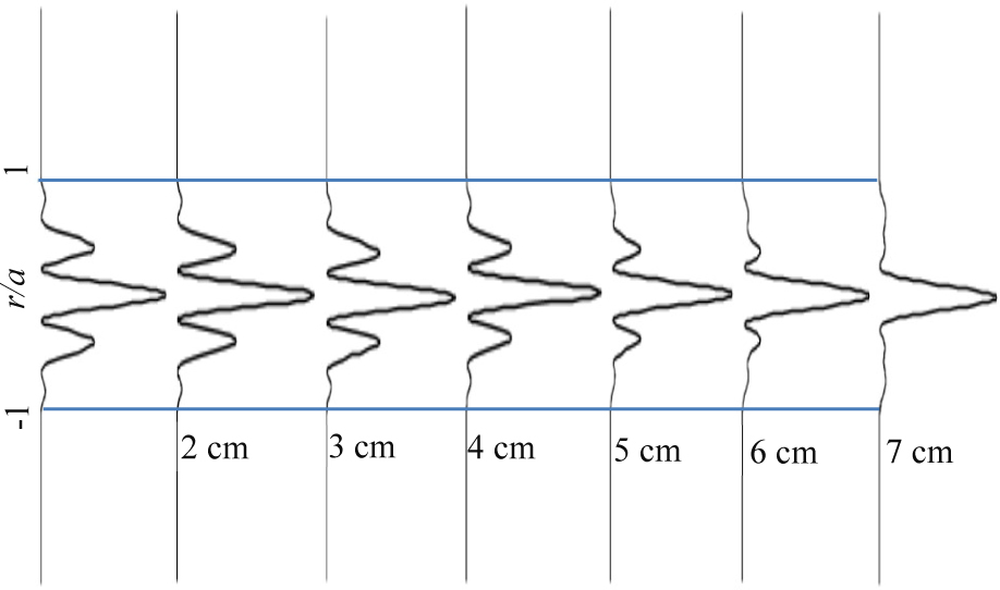
Figure 5: Transverse intensity patterns at different positions inside an optical waveguide of length L = 7 cm and a = 0.6 mm.

C Rule for mode coupling at the waveguide exit plane

Here, the set of waveguide modes must be coupled to a set of free space modes. The field at the left side of the waveguide exit plane is

$$E_3\left(r\right)=\sum _{n=1}^{n_3}{\mathrm{CG}}_n{\mathrm{EH}}_n(r),$$

(9)

where the integer $n_3$ is the number of the waveguide modes, which is equal to $n_2$obtained from eqn (7), and the ${\mathrm{CG}}_{\mathrm{n}}$ coefficients are calculated usingeqn (2.2).

The field at the right side of the waveguide exit plane is

$$E_4\left(r\right)=\sum _{m=1}^{n_4}{C}_m{\mathrm{TEM}}_m(r),$$

(10)

where $C_m$ are defined in eqn (6) and the integer $n_4$ is the considered number of the TEM modes.

Table 2 shows, for each given number ${\mathit{\text{n}}}_3$ of the used waveguide modes, the optimum number $n_4$ of free space modes which allows an efficient mode coupling at the waveguide exit plane. This result is achieved for different w/a ratios.

Table 2: Optimized number $n_4$ of free space modes as a function of the number $n_3$ of the used waveguide modes

${\mathit{\text{n}}}_{\mathbf{3}}$	${\mathit{\text{n}}}_{\mathbf{4}}$
7	16
8	21
9	29
10	36
11	40
12	55
14	70
17	100
19	130
22	175
25	219
30	316

The plot $n_4$ versus $n_3$ is illustrated by the point curve in Figure 6.

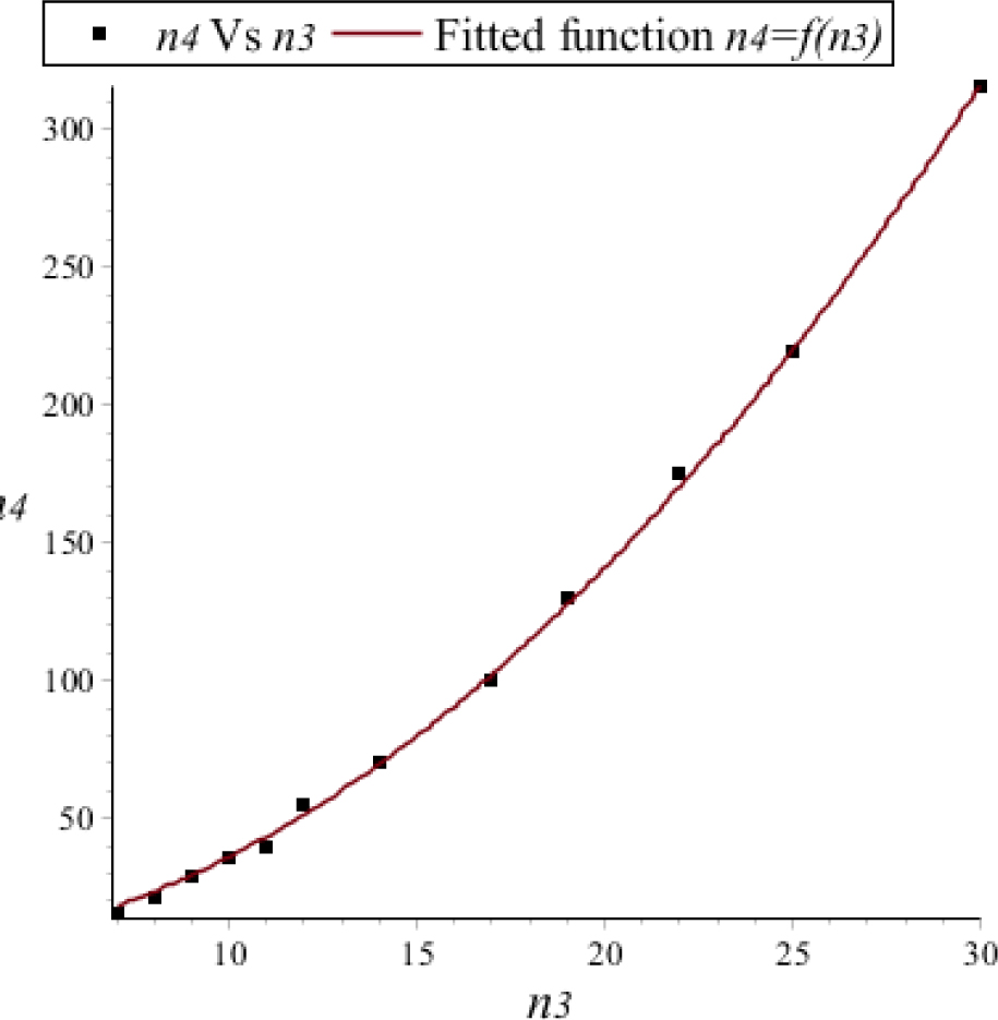
Figure 6: Optimized number $n_4$ of free space modes as a function of the number $n_3$ of the used waveguide modes.

Applying the mathematical fit instructions of Maple software, using the data from Table 2, the appropriate function $n_4=f(n_3)$ is deduced and the following rule for mode coupling at the waveguide exit plane isobtained:

$$n_4=\lfloor 0.35n_3^2+1\rfloor .$$

(11)

Figure 7 shows mode coupling according to this rule for different values of$n_3$.

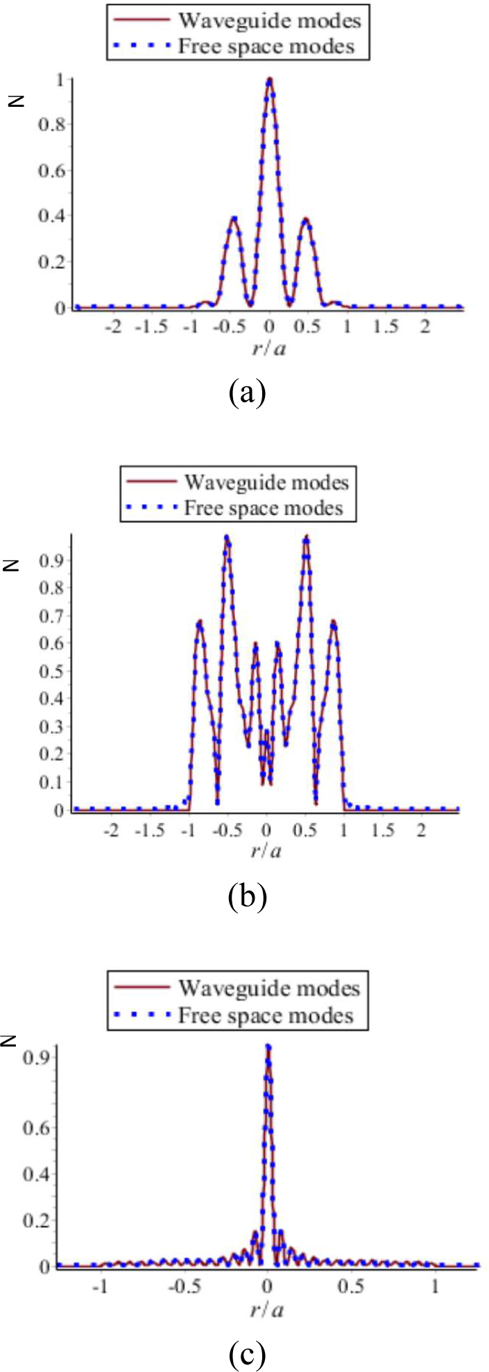
Figure 7: Superposition of transverse field distribution at the waveguide exit plane with a = 0.6 mm for (a) n${}_{\mathrm{3}}$ = 7, (b) n${}_{\mathrm{3}}$ = 10, and (c) n${}_{\mathrm{3}}$ = 25.

The results shown in Figure 7 (a)–(c) have been computed with w/a = 0.58, w/a = 0.5, and w/a = 0.8, respectively. As mentioned in Section II-A, we confirm that for each case, and thanks to the rule, an efficient mode coupling has been verified for other arbitraryratios w/a.

It should be noted that at both ports of the waveguide and according to the rule, mode coupling goes successfully independent of the ratio w/a for values outside the range 0.45 $<$ w/a $\mathrm{<}$ 0.73 applied by different authors [10–14]. Indeed, the rule works very well at least in the range 0.3 $<$ w/a $\mathrm{<}$ 0.9 which is moreuseful.

D Field beyond the optical waveguide

Propagation through free space beyond the waveguide of the emerged field considered in Figure 7 is shown in Figure 8.

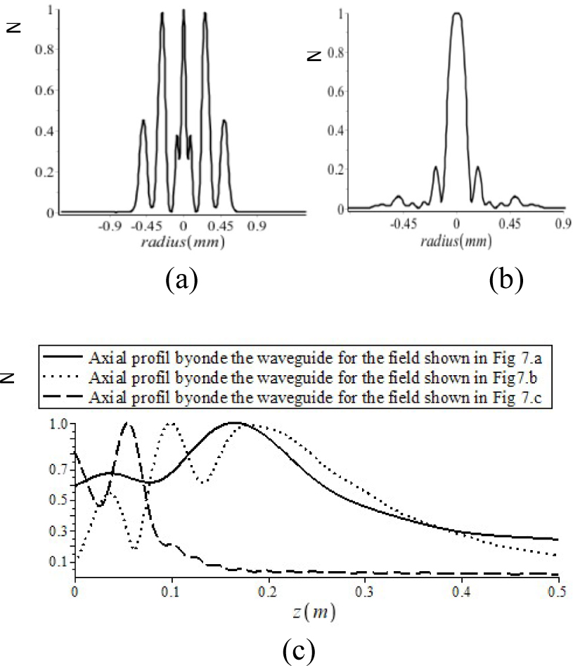
Figure 8: Transverse distribution of the field shown in Figure 7 (b) at (a) z = 15 mm and (b) z = 95 mm beyond the optical waveguide, respectively, and (c) axial field distribution for the fields shown in Figure 7.

We underline that beyond the waveguide, propagation through any optical path, composed by an apertured first-order optical system, can be achieved using the ABCD law and the generalized Gouy phase (GGP) shift [16–19].

III. CONCLUSION

In this paper, waveguide crossing has been solved by giving a simple rule for an efficient mode coupling at both ends of a cylindrical optical waveguide. Using the optimum number of modes given by the rule, crossing of the optical waveguide is achieved successfully regardless of the constraint of the ratio between the beam spot size and the waveguide radius.

REFERENCES

[1] Q. Wu, J. Zhang, Y. Yang, and X. Shi, “The temperature compensation for TE011 mode resonator with bimetal material,” Applied Computational Electromagnetic Society (ACES) Journal, vol. 34, no. 07, pp. 1070-1075, Jul. 2019.

[2] M. Stefszky, R. Ricken, C. Eigner, V. Quiring, H. Herrmann, and C. Silberhorn, “Waveguide cavity resonator as a source of optical squeezing” Phys. Rev Applied, vol. 7, pp. 044026, 2017.

[3] S. Pachnicke, Fiber-Optic Transmission Networks: Efficient Design and Dynamic Operation, Springer-Verlag Berlin Heidelberg, 2012.

[4] $\acute{\mathrm{A}}$. A. San-Blas and J. M. Roca, “Highly efficient technique for the full-wave analysis of circular waveguide filters including off-centered irises,” Applied Computational Electromagnetic Society (ACES) Journal, vol. 30, no. 11, pp. 1230-1240, Nov. 2015.

[5] R. G. Hunsperger, Integrated Optics Theory and Technology. Sixth Edition, Springer-Verlag New York.2009.

[6] E. A. J. Marcatili and R. A. Schmeltzer, “Hollow metallic and dielectric waveguides for long distance optical transmission and lasers,” Bell Syst. Tech. J., vol. 43, pp. 1783-1809, 1964.

[7] J. J. Degnan, “The waveguide laser, A review,” Appl. Phys., vol. 11, pp. 1-33, 1976.

[8] R. L. Abrams, “Coupling losses in hollow waveguide laser resonators,” IEEE J. Quantum Electron., vol. QE-8, pp. 838-843, Nov. 1972.

[9] Y. Wong and N. H. Hiraguri, “Attenuation in lossy circular waveguides,” Applied Computational Electromagnetic Society (ACES) Journal, vol. 34, no. 1, pp. 43-48, Jan. 2019.

[10] P. W. Smith, “A waveguide gas laser,” Appl. Phys. Lett, vol. 19, pp. 132-134, 1971.

[11] F. P. Roullard III and M. Bass, “Transverse mode control in high gain, millimeter bore, waveguide lasers,” IEEE J. Quantum Electron., vol. QE-13, pp. 813-819, Oct. 1977.

[12] R. L. Abrams and A. N. Chester, “Resonator theory for hollow waveguide lasers,” Appl. Opt., vol. 13, pp. 2117-2125, 1974.

[13] M. TACK, “The influence of losses of hollow dielectric waveguides on the mode shape,” Journal of Quantum Electronics, vol. QE-18, pp. 2022-2026, 1982.

[14] R. Gerlach, D. Wei, and N. Amer, “Coupling efficiency of waveguide laser resonators formed by flat mirrors: Analysis and experiment,” IEEE Journal of Quantum Electronics, vol. Qe-20, no. 8, pp. 948-963, 1984.

[15] H. Kogelnik, “Coupling and conversion coefficients for optical mode,” in Proc. Symp. Quasi-Optics, J. Fox, Ed, Brooklyn, NY: Polytechnic Press, pp. 333-347, 1964.

[16] H. Kogelnik and T. Li, “Laser beams and resonators,” Proc. IEEE, vol. 5, no. 4, pp. 1312-1329, 1966.

[17] A. E. Siegman, Lasers, University Science Books Mill Valley, California (1986).

[18] Z. Derrar Kaddour, A. Taleb, K. Ait-Ameur, and G. Martel, “Revisiting gouy phase,” Optics Communications, vol. 280, pp. 256-263, 2007.

[19] Z. Derrar Kaddour, A. Taleb, K. Ait Ameur, G. Martel, and E. Cagniot, “Alternative model for computing intensity patterns through apertured ABCD systems,” Optics Communications, vol. 281, pp. 1384-1395, 2008.

BIOGRAPHIES

Billel Bentouhami received the engineering degree in physics from the University of Ferhat Abbes, S$\acute{\mathrm{e}}$tif, Algeria, in 2009 and the Magister degree in quantum electronics from the University of Sciences and Technology Houari Boumedi$\acute{\mathrm{e}}$ne (USTHB), Algeria, in 2012. He is currently working toward the Ph.D. degree with the University of Sciences and Technology Houari Boumedi$\acute{\mathrm{e}}$ne.

He is a member of the Quantum Electronics Laboratory LEQ of USTHB and is presently an Assistant Professor of Physics with the University of Bordj Bou Arreridj, Algeria. His research interests include optical waveguides, diffraction, electromagnetic field propagation and quantum electronics.

Zaia Derrar Kaddour received the Ph.D. degree in physics from the University of Sciences and Technology Houari Boumedi$\acute{\mathrm{e}}$ne, Algeria, in 2007.

She is a member of Quantum Electronics Laboratory LEQ and an OSA member. She is currently a Professor of Physics with the University of Sciences and Technology Houari Boumedi$\acute{\mathrm{e}}$ne, Algeria. Her current research interests include optical resonators, electromagnetics field propagation, and optics.

ACES JOURNAL, Vol. 37, No. 5, 648–653.
doi: 10.13052/2022.ACES.J.370515
© 2021 River Publishers

Abstract

I. INTRODUCTION

II. THEORY AND NUMERICAL RESULTS

A Rule for mode coupling at the waveguide entrance plane

B Propagation inside the waveguide

C Rule for mode coupling at the waveguide exit plane

D Field beyond the optical waveguide

III. CONCLUSION

REFERENCES

BIOGRAPHIES