FDTD Simulations of Modulated Metasurfaces with Arbitrarily Shaped Meta-atoms by Surface Impedance Boundary Condition
Yanmeng Hu, Quanen Zhou, Xinyu Fang, and Mengmeng Li
Department of Communication Engineering
Nanjing University of Science and Technology, Nanjing, 210094, China
limengmeng@njust.edu.cn
Submitted On: January 18, 2021; Accepted On: July 7, 2021
Abstract
In this paper, we propose a reduced-complexity finite difference time domain (FDTD) simulations of modulated metasurfaces with arbitrary unit cells. The three dimensional (3D) physical structure of the metasurface is substituted by a spatially varying surface impedance boundary condition (IBC) in the simulation; as the mesh size is not dictated by sub-wavelength details, considerable advantage in space- and time-step is achieved. The local parameters of the IBC are obtained by numerical simulation of the individual unit cells of the physical structure, in a periodic environment approximation, in the frequency domain. As the FDTD requires an appropriate time domain impulse-response, the latter is obtained by broad-band frequency simulations, and vector fitting to an analytic realizable time response. The approach is tested on metasurface structures with complex unit cells and extending over 10 10 wavelengths, using a standard PC with 64GB RAM.
Index Terms: thin-layer model, metasurface, FDTD, impedance boundary condition.
I. INTRODUCTION
Metasurfaces are thin-layer arrays composed of the so called “electromagnetic meta-atoms,” which have been proved to allow unprecedented electromagnetic field manipulations [1, 2]. Due to their advantages of low profile, low cost, easy fabrications, and diverse strategies for realizations, many applications have been reported, such as: radar cross section (RCS) reduction [3], low-scattering antennas [4], planar antennas [5], lenses [6], [7], imaging [8], etc.
The meta-atoms are sub-wavelength in size, and likewise closely spaced; the resulting structure is thus electrically thin, while typically extending over several wavelengths in size; very often, the field manipulation requires meta-atoms with complicated structures. As a result, it is challenging to simulate such multiscale problems with dense discretization and large electrical size by full-wave methods [2], [9], [10].
Most types of field manipulation require that the metasurface be spatially varying over its surface; however, this variability is on the order of the wavelength, i.e. slow with respect to the size of meta-atoms (hence the term “modulated” often employed). Therefore, homogenization yields accurate results, and the effects of sub-wavelength atoms is well described in terms of surface impedance boundary conditions (IBCs) [2], [11, 12, 13], that can take different forms [14, 15, 16, 17, 18, 19, 20, 21, 22, 23, 24, 25, 26]. This consideration allows a significant reduction of computational load for full-wave analysis; of course it requires that the problem formulation be consistent with the field boundary conditions employed to homogenize the sub-wavelength atoms collectively. In most applications, the underlying lattice of the atoms remains regular, or weakly varying; this allows to use the periodic-medium approximation in relating the surface impedance to the features of the individual meta-atoms.
In this short paper, we propose an FDTD method with surface impedance boundary condition (IBC) for the simulations of spatially varying (i.e. modulated) metasurfaces. Specifically, we address the case of meta-atoms with arbitrary shapes, for which no analytical expression can be found of the equivalent surface impedance. We propose a method to insert numerical characterization of the IBC into the scheme, including the necessity to properly account for frequency dispersion in the time response. The IBC approach reduces mesh density in the longitudinal direction by virtue of homogenization into an IBC [24], by de facto removing the meta-atom thickness. However, we would like to stress that in our approach we use the nature of modulation to likewise reduce the necessary mesh density in the transverse directions, as modulations are on the order of the wavelength.
To the best of the authors’ knowledge, this use of numerically-derived IBC to solve both thickness and transverse meshing issues is novel in FDTD, and applied for the first time to large metasurfaces.
The rest of this paper is organized as follows: in Section II, the background of IBC and FDTD is summarized; in Section III, the numerical homogenization for wideband full-wave FDTD simulation of metasurface is proposed; numerical results and discussions in Section IV demonstrate the validity of the proposed method. Finally, a brief conclusion is given in Section V.
II. BACKGROUND
A. Impedance boundary condition (IBC)
When a surface impedance boundary condition is appropriate, the total transverse electric and magnetic fields on the concerned surface are linked as [11, 12, 13]
| (1) |
where and are the fields on the outer side of the metasurface, and is the equivalent surface impedance, in general of tensor nature. We have explicitly denoted frequency dependence to recall that this is naturally a frequency domain description, while in the following we will address time-domain solution of Maxwell equations. The one-sided description of the homogenized structure in (1) avoids meshing the dielectric (where FDTD would have meshing problems), and is appropriate for thin layers (where spatial dispersion is negligible). Structural symmetry in the meta-atoms generates isotropy in the boundary conditions, and the effective surface impedance is scalar, so that
Analytic expressions of the surface impedance can be obtained only for a few simple unit cells [26]. In this paper, we consider meta-atoms with arbitrary structure, and the surface impedances will be extracted from numerical simulation of the meta-atom unit cells, as described below in Secs. III and IV.
B. FDTD with frequency dispersion
In this paper, we follow the classical Yee cell FDTD [27, 28, 29, 30], and the usual leap-frog scheme. We will also use FDTD with 2D- or 1D-periodic boundary conditions, which implement the method in [36]. As FDTD is time-domain, it is necessary to express the linear IBC (1) as a time convolution:
where now Z(t) represents the impulse responses, i.e. the Fourier (back) transforms of their frequency-domain counterparts in eqn (1).
In the following we will resort to approximations of the dispersion that allow for closed-form expressions of the impulse responses in eqn (3). The piecewise linear recursive convolution (PLRC) method [31] will be employed to evaluate the convolutions in eqn (3). The updating equations for computation domains not involved in the IBC surface are same as the standard FDTD [27, 28, 29, 30].
III. NUMERICAL HOMOGENZATION
A. Surface impedance extraction from numerical simulation of meta-atoms
As alluded in the Introduction, we will obtain the local values of the (spatially variable) surface impedance via numerical simulation of the local meta-atoms. We will employ the periodicity approximation, which accounts for inter-element coupling, and that has been successfully used in the design of metasurface cells as reported in several publications [1, 2, 3, 4, 5, 6, 7, 8]. Here we will call “unit cell” the meta-atom in the periodic lattice; because of the periodic approximation, the simulation is better performed in the frequency domain. The simulation of the unit cell can be carried out with several approaches, most usually finite-elements (FEM) and Method of Moments (MoM); here we will use FEM as implemented in the commercial software HFSS.
In order to reduce the associated numerical cost, we will resort to a method that allows wide-angle response with a limited number (two) of simulations [2], [20]. While the method is general, for the sake of illustration we will consider isotropic meta-atoms constituted by close ring resonators (CRRs) [32] on a grounded dielectric substrate, as in Figure 1.
The approach is based on separating the metal layer (here, the ring) from the grounded slab; as the metal features are sub-wavelength and non-resonant, both their frequency and spatial dispersion (dependence on incidence angle) are weak; as typically higher Floquet modes are deeply evanescent, the equivalent modal circuit is as depicted in Figure 2. As mentioned earlier, we consider explicitly symmetric meta-atoms, which yield an isotropic impedance, and no TE-TM coupling; more general situations are readily accounted for by this coupling and modal network slightly more complex than in Figure 2.
The wide-angle response of the metal feature (ring, here) is conveniently expressed using the generalized sheet transition condition (GSTC) description of the boundary condition [2], [20], i.e. in terms of polarization susceptibility tensors. This yields an expression valid for any incidence angle that however requires only computation of the response for two angles: normal incidence , and one oblique incidence encompassing the incidence angle range of interest [2], [20].
The polarization susceptibilities are then expressed in terms of the reflection (R) and transmission (T) coefficients as:
| (4) |
| (5) |
where denotes the wave number in free space, and the transmission and reflection coefficients at normal incidence, and are the transmission and reflection coefficients for incidence angle . The indication of TM or TE polarization has been assumed and omitted in the susceptibilities to avoid notation cluttering, and likewise in reflection (R) and transmission (T) coefficients. One can then pass to the impedance format of the IBC via the following relationships [25]:
| (6a) |
| (6b) |
where , , , and denote the surface impedances of TE and TM polarized plane wave at an oblique incidence angle , respectively; note that terms in the equations above are also TE and TM although that is not explicitly indicated.
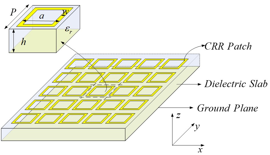
Figure 1: Example of meta-atoms in a periodic environment: CRR meta-atoms.
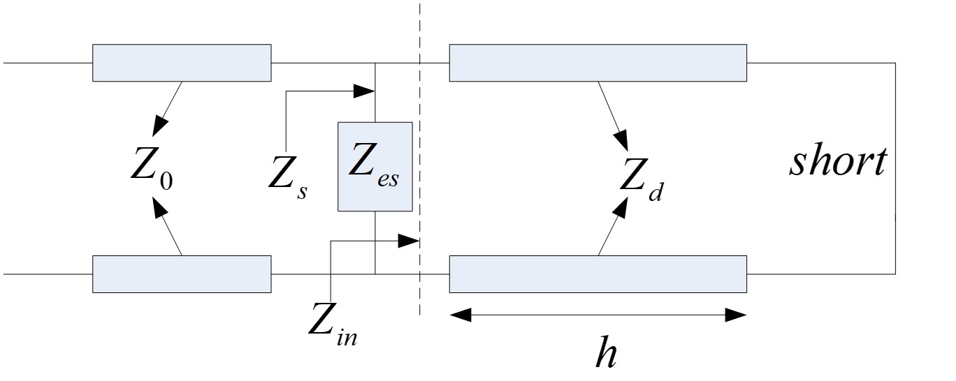
Figure 2: Equivalent modal transmission line circuit model of the meta-atoms under periodic boundary conditions.
The surface impedances required in eqn (3) are then obtained via the equivalent modal transmission line circuit in Figure 2:
| (7) |
where , and are the characteristic impedances of free space and the dielectric,
| (8) |
| (9) |
For metasurfaces with non-uniform meta-atoms and thus space-varying surface impedance, the projection from the physical structure to its surface impedance description is depicted in Figure 3, where the meta-atoms are substituted by a cell of surface impedance, with values computed as described above. As a result, the metasurface thickness is not meshed at all, and the transverse FDTD mesh density is dictated only by the spatial variability of the meta-atoms (e.g. modulation), which is on the scale of the wavelength; this drastically increases the simulation efficiency of the modulated metasurface; in FDTD, this is even more pronounced than in frequency-domain methods, as time step is related to space discretization by stability, as well known (e.g. [33]).
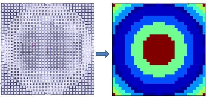
Figure 3: Modulated metasurface with non-uniform complicated meta-atoms and the corresponding surface impedance.
B. Full-wave simulation with dispersive FDTD
For wideband full-wave simulations of the modulated metasurface, the surface impedances derived in eqn (6) and (7) have complicated relationship with frequency, which cannot be inserted into FDTD directly. As a result, we fit the frequency response with a model that allows closed-form time-domain expressions. As we expect resonances across the bandwidth of interest because of the nature of the meta-atom itself, we employ the following model:
| (10) |
where is a constant real number, is the order ofrational function, and are residue and pole, respectively. The expression above is fit to the actual frequency response (deriving from numerical simulations) via the vector fitting method [34], in which the nonlinear approximation in eqn (10) can be evaluated with two stages of linear problems.
The time domain expressions read:
| (11) |
Since has an exponential form, the convolution integrals can be easily solved by the recursive convolution method [35]. Take for example, the surface impedance boundary condition at the cell is discretized with FDTD as
where
IV. NUMERICAL RESULTS AND DISCUSSION
In this section, numerical examples are presented to validate the accuracy and efficiency of the proposed scheme. In all examples, the incidence angle in eqn (4) and (5) is chosen to, which has shown to provide good results in all cases: it is chosen as a tradeoff with respect to the impact of in the denominator of eqn (5) [2], [20]. The proposed algorithm was implemented single thread with Intel Fortran 64-bit compiler, all the computations were carried out on the same computer with an Intel (R) Core (TM) i7-8700 CPU @3.7GHz and 64 GB RAM. The logic here is progressive: (1) first we validate the method against a fully periodic structure (2D periodicity, infinitely extended); (2) we validate on a 1D periodic case, i.e. with periodic boundary conditions along one direction; and (3) we finally show application to a fully 2D variation of the impedance.
A. Uniform infinite metasurface sheet (Meta-atom under periodic boundary conditions)
As a first test, we compare the FDTD-IBC against a standard FDTD and HFSS in a periodic environment. The results are shown in Figure 4, which reports the reflection coefficient phase and amplitude of the CRR meta-atom of Figure 1 from 5 GHz to 10 GHz (note inclusion of nominal substrate losses). The excellent agreement proves the accuracy of the proposed method. Table I lists the necessary grids size, and the related computational requirements, showing significant savings of both the computation time (218 s to 2 s) and memory (128.5 MB to 4.7 MB), which demonstrate the validity of the proposed FDTD-IBC.
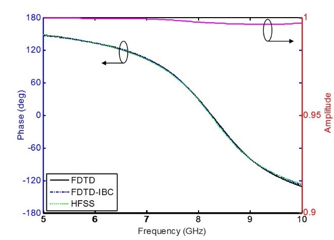
Figure 4: Accuracy validation: wideband reflection phase and amplitude with (2D) periodic boundary conditions, for the CRR meta-atom shown in Figure 1, with , , , , and (note that substrate losses are included).
Table 1: Computation performance comparison of FDTD and FDTD-IBC for the wideband simulation of CRR meta-atom
| Grid size | Time | Memory | |
|---|---|---|---|
| (s) | (MB) | ||
| FDTD | 218 | 128.5 | |
| FDTD-IBC | 2 | 4.7 |
B. Wideband reflection field manipulations with gradient metasurface (1D periodicity)
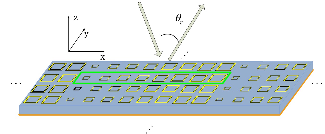
Figure 5: Gradient metasurface for reflection fields manipulations, the reflection angle for a given incidence angle is determined by the phase gradient along .
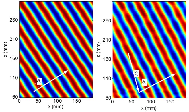
Figure 6: Validation: reflection fields manipulations by the gradient metasurface at 7.5 GHz under (a) normal incidence, (b) oblique incidence , both of the simulated reflection angles agree well with the analytical values by generalized reflection law [1].
Table 2: Parameters of the 3 bit CRR meta-atoms for reflection fields manipulations at 7.5 GHz
| Meta-atoms |
1 | 2 | 3 | 4 | 5 | 6 | 7 | 8 |
|---|---|---|---|---|---|---|---|---|
| a (mm) | 3.01 | 4.82 | 5.13 | 5.32 | 5.44 | 5.54 | 5.72 | 5.92 |
| Meta-atoms |
1 | 2 | 3 | 4 | 5 | 6 | 7 | 8 |
| a (mm) | 3.65 | 5.80 | 6.25 | 6.53 | 6.72 | 6.92 | 7.22 | 7.90 |
Table 3: Computation performance comparison of FDTD and FDTD-IBC for wideband simulation of gradient metasurface.
| Number of grids | Time | Memory | |
|---|---|---|---|
| FDTD | 50.1 h | 27.7 GB | |
| FDTD-IBC | 314 s | 639.2 MB |
Next, we examine a practical example of metasurface device, yielding the so-called non-Snell reflection via a gradient-phase metasurface, adopting the structure in [1]. For a plane wave with incidence angle , the reflection angle from the designed gradient metasurface will follow the generalized law ofreflection [1]
| (13) |
where , is the designed phase gradient along . Here we consider periodicity along the y direction. Table II lists the relevant geometric parameters for the reported test cases.
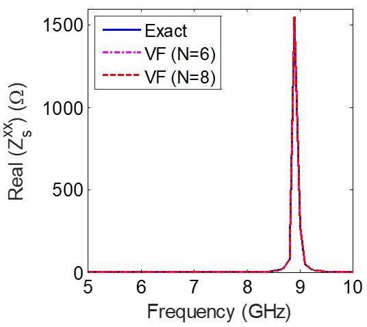
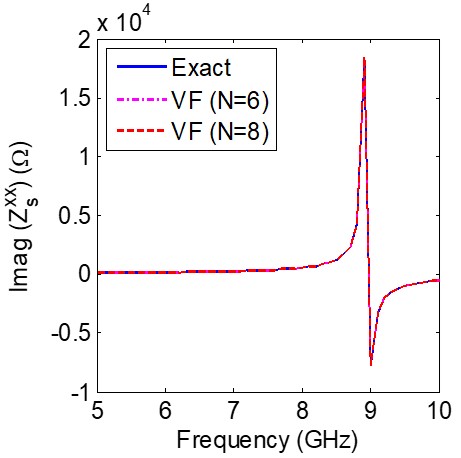
Figure 7: Vector fitting (VF) for the surface impedances from 5 GHz to 10 GHz for the CRR with mm, (a) real part, (b) imaginary part.
At first, we simulate the reflection fields from the gradient metasurface under normal incidence. Figure 6 (a) shows the simulated reflection fields at 7.5 GHz, the period of the meta-atom is 6 mm. The meta-atoms of number 1 to 8 in Table II are placed along with a constant phase difference of ; the length of the metasurface is , corresponding to , and the y-period is 6 mm. The reflection angle simulated by FDTD-IBC is, which agrees well with the analytical value of evaluated by eqn (13). Then, we simulate the reflection fields under oblique incidence angle of as in Figure 6 (b), the period of the meta-atom is 8 mm, the same number of meta-atoms listed in Table II is employed. The reflection angle simulated by FDTD-IBC is, which agrees well with the analytical value of evaluated by eqn (13).
For wideband simulations, the surface impedance should be fitted as explained in Sec. III-B. Figure 7 shows the wideband surface impedances of the CRR meta-atom when mm of exact data and vector fitting method [34]. It can be concluded that when and , the fitted surface impedance converges to the exact data. We choose in the following simulations, as they employ the same meta-atoms.
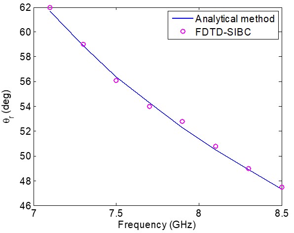
Figure 8: Wideband simulated reflection angle of the gradient metasurface with eqn (13) and FDTD-IBC from 7.1 GHz to 8.5 GHz.
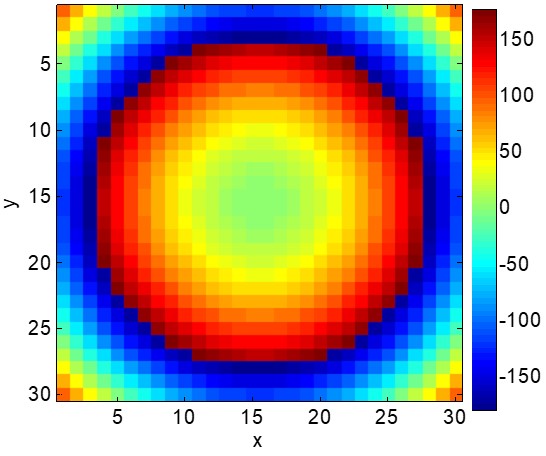
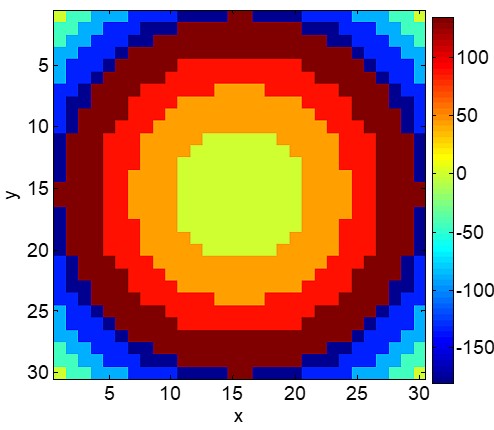
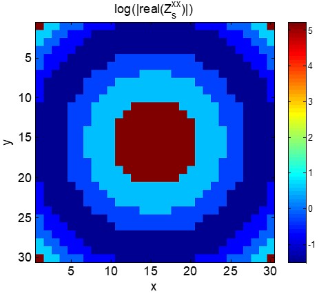
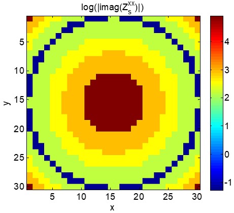
Figure 9: Phase distributions of the metareflector for reflection fields focusing at 7.5 GHz with the CRRs, (a) GO target phase [1], (b) phase compensation with 3 bit meta-atoms, (c) , (d) .
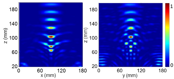
Figure 10: Normalized focusing fields of the metareflector A i.e. at 7.5 GHz, (a) xoz plane, (b) yoz plane.
Figure 8 shows the reflection angle from 7.1 GHz to 8.5 GHz for the gradient metasurface in Figure 6 (a) evaluated by generalized reflection law [1] and the proposed FDTD-IBC, very good agreements between them can be found. Table III lists the computation time and memory requirements for the wideband simulation of gradient metasurface. The discretization sizes for FDTD and FDTD-IBC are 0.1 mm and 1mm, respectively, showing the potential for larger surfaces; in this case computation time is reduced from 50.1 hours to 314 seconds, and the memory is reduced from 27.7 GB to 639.2 MB.
C. Reflection fields focusing with 2D metasurface (Metareflector)
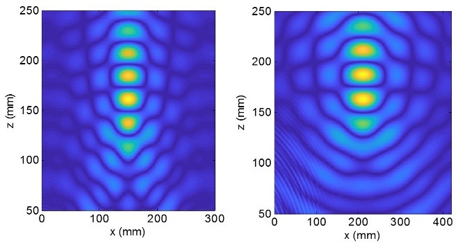
Figure 11: Normalized focusing fields of xoz plane by the metareflectors B and C at 7.5 GHz, i.e. (a) , with meta-atoms and (b) , with meta-atoms.
As a final application example, we consider a metasurface with two-dimensional variation, designed for reflection field focusing for normal plane-wave incidence. We will call “metareflector” this structure, in analogy to the cognate reflectarrays. The phase distribution is based on the Geometrical Optics (GO) approximation, yielding
| (14) |
for a focal length ; the surface impedance is again designed so as to yield the desired phase. Figure 9 shows the resulting structure for =180 mm at 7.5 GHz; Figure 9 (a) plots the ideal (continuous) GO phase compensation at the location of , and Figure 9 (b) the realized phase distributions with 3 bit CRR meta-atoms. The effective surface impedances distributions of the metareflector are obtained from the precomputed meta-atoms listed in Table II as in Figure 9 (c) and (d). The physical structures of the metareflector are substituted by homogeneous surface impedances as indicated earlier.
We consider three diameters: (A) , i.e. 4.5 wavelengths at the operating frequency, and ; (B) , i.e. 7.5 wavelengths, and ; (C) , i.e. 10.5 wavelengths, and . Figure 10 and Figure 11 show the normalized reflection field manipulations by the designed metasurface reflector at the xoz and yoz plane. For the relatively small structure A in Figure 10, there is a significant discrepancy between the planned focal length (180 mm) and the observed one, 109 mm; this is to be expected from a GO-based design. Indeed, the situation changes with larger sizes, of 7.5 and 10.5 wavelengths, as seen in Figure 11 yielding 161 and 175 mm focal lengths, respectively, thus actually nearing the GO prediction [37]. Table IV lists the computation time and memory requirements for the full wave simulations of the proposed method, where the discretization sizeis 0.5 mm.
Table 4: Computation time and memory performance of the FDTD-IBC for metareflectors of different dimensions
| Type | Number of | Dimensions | Number | Time | Memory |
| meta-atoms | [] | of grids | [h] | [GB] | |
| A | 0.39 | 12.5 | |||
| B | 1.75 | 32.6 | |||
| C | 3.34 | 54.7 |
V. CONCLUSION
In this short paper, we have presented and validated an effective surface impedance boundary condition (IBC) for FDTD for wideband simulations of modulated metasurface with complicated meta-atoms. The local surface impedance is obtained via frequency domain (FEM) simulation of the meta-atoms in the periodic approximation, and vector fitting method for the frequency dependence not get closed-form time domain impulse responses. With the proposed method, the thickness of the metasurface is not discretized in the FDTD, and the transverse variation only requires space discretization to match the modulation, which is slow. Hence, the multiscale metasurface can be substituted by homogenous surface impedance, and the number of unknowns is reduced significantly. Examples of metasurfaces for reflected field manipulations are shown to demonstrate the validity of the proposed method.
ACKNOWLEDGMENT
This work was supported in part by Natural Science Foundation of China under Grant 61871222 and 61890541, the Fundamental Research Funds for the Central Universities of 30921011101.
REFERENCES
[1] N. Yu and F. Capasso, “Flat optics with designer metasurfaces,” Nature Materials, vol. 13, no. 2, pp. 139-150, 2014.
[2] C. L. Holloway, E. F. Kuester, J. A. Gordon, J. O’Hara, J. Booth, and D. R. Smith, “An overview of the theory and applications of metasurfaces: the two-dimensional equivalents of metamaterials,” IEEE Antennas Propag. Mag., vol. 54, no. 2, pp. 10-35, Feb. 2012.
[3] S. Zhou, X. Fang, M. Li, and R. S. Chen, “S/X dual-band real-time modulated frequency selective surface based absorber,” Acta Physica Sinica, vol. 69, no. 20, pp. 204101, 2020.
[4] Y. Liu, K. Li, Y. Jia, Y. Hao, S. X. Gong, and Y. J. Guo, “Wideband RCS reduction of a slot array antenna using polarization conversion metasurfaces,” IEEE Trans. Antennas Propag., vol. 64, no. 1, pp. 326-331, Jan. 2016.
[5] G. Minatti, F. Caminita, M. Casaletti, and S. Maci, “Spiral leakywave antennas based on modulated surface impedance,” IEEE Trans. Antennas Propag., vol. 59, no. 12, pp. 4436-4444, Dec. 2011.
[6] M. Li, S. Li, Y, Yu, X, Ni, and R. S. Chen, “Design of random and sparse metalens with matrix pencil method,” Opt. Express, vol. 26, no. 19, pp. 24702-24711, Sep. 2018
[7] M. Li, S. Li, L. K. Chin, Y. F. Yu, D. P. Tsai, and R. S. Chen, “Dual-layer achromatic metalens design with an effective Abbe number,” Opt. Express, vol. 28, no. 18, pp. 26041-26055, Aug. 2020
[8] L. Li, H. Ruan, C. Liu, Y. Li, Y. Shuang, A. Alù, and T. J. Cui, “Machine-learning reprogrammable metasurface imager,” Nature Communications, vol. 10, no. 1, pp. 1082, 2019.
[9] C. L. Holloway, A. Dienstfrey, E. F. Kuester, J. F. OHara, A. K. Azad, and A. J. Taylor, “A discussion on the interpretation and characterization of metafilms/metasurfaces: the two-dimensional equivalent of metamaterials,” Metamaterials, vol. 3, no. 2, pp. 100-112, 2009.
[10] Y. Guo, T. Zhang, W. Y. Yin, and X. H. Wang, “Improved hybrid FDTD method for studying tunable graphene frequency-selective surfaces (GFSS) for THz-wave applications,” IEEE Trans. Terahertz Sci. Technol., vol. 5, no. 3, pp. 358-367, May 2015.
[11] J. G. Maloney, G. S. Smith, “The use of surface impedance concepts in the finite-difference time-domain method,” IEEE Trans. Antennas Propag., vol. 40, no. 1, pp. 38-48, Jan. 1992.
[12] M. A. Francavilla, E. Martini, S. Maci, and G. Vecchi, “On the numerical simulation of metasurfaces with impedance boundary condition integral equations,” IEEE Trans. Antennas Propag., vol. 63, no. 5, pp. 2153-2161, May 2015.
[13] B. Stupfel and D. Poget, “Sufficient uniqueness conditions for the solution of the time harmonic maxwell’s equations associated with surface impedance boundary conditions,” J. Comput. Phys., vol. 230, no. 12, pp. 4571-4587, Jun. 2011.
[14] E. F. Kuester, M. A. Mohamed, M. Piket-May and C. L. Holloway, “Averaged Transition Conditions for Electromagnetic Fields at a metafilm,” IEEE Trans. Antennas Propag., vol. 51, no. 10, pp. 2641-2651, Oct. 2003.
[15] C. L. Holloway, D. C. Love, E. F. Kuester, J. A. Gordon, and D. A. Hill, “Use of generalized sheet transition conditions to model guided waves on metasurfaces/metafilms,” IEEE Trans. Antennas Propag., vol. 60, no. 11, pp. 5173-5186, Nov. 2012.
[16] D. González-Ovejero and S. Maci, “Gaussian ring basis functions for the analysis of modulated metasurface antennas,” IEEE Trans. Antennas Propag., vol. 63, no. 9, pp. 3982-3993, Sep. 2015.
[17] M. Bodehou, D. Gonzalez-Ovejero, C. Craeye, and I. Huynen, “Method of moments simulation of modulated metasurface antennas with a set of orthogonal entire-domain basis functions,” IEEE Trans. Antennas Propag., vol. 67, no. 2, 1119-1130, Feb. 2018.
[18] M. Bodehou, C. Craeye, and I. Huynen, “Electric field integral equation-based synthesis of elliptical-domain metasurface antennas,” IEEE Trans. Antennas Propag., vol. 67, no. 2, pp. 1270-1274, Feb. 2019.
[19] Q. Wu, “Characteristic mode analysis of composite metallic–dielectric structures using impedance boundary condition,” IEEE Trans. Antennas Propag., vol. 67, no. 12, pp. 7415-7424, Dec. 2019.
[20] K. Achouri, M. A. Salem, and C. Caloz, “General metasurface synthesis based on susceptibility tensors,” IEEE Trans. Antennas Propag., vol. 63, no. 7, pp. 2977-2991, Jul. 2015.
[21] C. Pfeiffer and A. Grbic, “Bianisotropic metasurfaces for optimal polarization control: Analysis and synthesis,” Phys. Rev. Appl., vol. 2, no. 4, p. 044011, Oct. 2014.
[22] X. Du, H. Yu, and M. Li, “Effective modeling of tunable graphene with dispersive FDTD-GSTC method,” Applied Computational Electromagnetics Society Journal, (Special Issue of ACES, Beijing, 2018), vol. 31, no. 6, pp. 851-856, 2019.
[23] X. Jia, F. Yang, X. Liu, M. Li, and S. Xu, “Fast nonuniform metasurface analysis in FDTD using surface susceptibility model,” IEEE Trans. Antennas Propag., vol. 68, no. 10, pp. 7121-7130, Oct. 2020.
[24] V. Nayyeri, M. Soleimani, O. M. Ramahi, “Modeling graphene in the finite-difference time-domain method using a surface boundary condition,” IEEE Trans. Antennas Propag., vol. 61, no. 8, pp. 4176-4182, May 2013.
[25] X. Liu, F. Yang, M. Li, and S. Xu, “Analysis of reflectarray antenna elements under arbitrary incident angles and polarizations using generalized boundary conditions,” IEEE Antennas Wirel. Propag. Lett., vol. 17, pp. 2208-2212, 2018.
[26] O. Luukkonen, C. Simovski, G. Granet, G. Goussetis, D. Lioubtchenko, A. V. Räisänen, and S. A. Tretyakov, “Simple and accurate analytical model of planar grids and high-impedance surfaces comprising metal strips or patches,” IEEE Trans. Antennas Propag., vol. 56, no. 6, pp. 1624-1632, Jun. 2008.
[27] K. Yee, “Numerical solution of initial boundary value problems involving Maxwell’s equations in isotropic media,” IEEE Trans. Antennas Propag., vol. 14, no. 3, pp. 302-307, May 1966.
[28] A. Taflove and S. C. Hagness, Computional Electrodynamics: The Finite-Difference Time-Domain Method, 3rd edition. Norwood, MA: Artech House, 2017.
[29] K. Niu, Z. X. Huang, M. Li, and X. L. Wu, “Optimization of the artificially anisotropic parameters in WCS-FDTD method for reducing numerical dispersion,” IEEE Trans. Antennas Propag., vol. 65, no. 12, pp. 7389-7394, Dec. 2017.
[30] K. Niu, Z. X. Huang, X. Ren, M. Li, B. Wu and X. L. Wu, “An optimized 3-D HIE-FDTD method with reduced numerical dispersion,” IEEE Trans. Antennas Propag., vol. 66, no. 11, pp. 6435-6440, Nov. 2018.
[31] D. F. Kelley and R. J. Luebbers, “Piecewise Linear Recursive Convolution for Dispersive Media Using FDTD,” IEEE Trans. Antennas Propag., vol. 44, no. 6, pp. 792-797, Jun. 1996.
[32] Y. Yang, L. Jing, B. Zheng, R. Hao, W. Yin, E. Li, C. M. Soukoulis, and H. Chen, “Full-polarization 3D metasurface cloak with preserved amplitude and phase,” Advanced Materials, vol. 28, no. 32, pp. 6866-6871, 2016.
[33] S. A. Cummer, “An analysis of new and existing FDTD methods for isotropic cold plasma and a method for improving their accuracy,” IEEE Trans. Antennas Propag., vol. 45, pp. 392-400, 1997.
[34] B. Gustavsen and A. Semlyen, “Rational approximation of frequency domain responses by vector fitting,” IEEE Transactions on Power Delivery, vol. 14, no. 3, pp. 1052-1061, Mar. 1999.
[35] R. Luebbers, F. P. Hunsberger, K. S. Kunz, R. B. Standler, and M. Schaneider, “A frequency-dependent time-domain formulation for dispersive materials,” IEEE Trans. Electromagn. Compat., vol. 37, pp. 222-227, Aug. 1990
[36] J. A. Roden, S. D. Gedney, M. P. Kesler, J. G. Maloney, and P. H. Harms, “Time-domain analysis of periodic structures at oblique incidence: Orthogonal and nonorthogonal FDTD implementations,” IEEE Trans. Microwave Theory Tech., vol. 46, pp. 420-427, Apr. 1998
[37] X. Li, S. Xiao, B. Cai, Q. He, T. J. Cui, and L. Zhou, “Flat metasurfaces to focus electromagnetic waves in reflection geometry,” Opt. Letters, vol. 37, no. 23, pp. 4940-4942, 2012.
BIOGRAPHIES

Yanmeng Hu received the B.S. degree in Electronic Information Science and Technology from the Henan University Minshen College, Kaifeng China, in 2017. She is pursuing the master’s degree in integrated circuit engineering in the Nanjing University of Science and Technology, Nanjing, China. Ms. Hu’s current research interest is electromagnetic analysis of multiscale problems.

Mengmeng Li received the B.S. degree (Hons.) in physics from Huaiyin Normal College, Huai’an, China, in 2007, and the Ph.D. degree in electromagnetic field and microwave technology from the Nanjing University of Science and Technology, Nanjing, China, in 2014. From 2012 to 2014, he was a Visiting Student
with the Electronics Department, Politecnico di Torino, Turin, Italy, and also with the Antenna and EMC Laboratory (LACE), Istituto Superiore Mario Boella, Turin, where he carried out fast solver for multiscale simulations. Since 2014, he has been with the Department of Communication Engineering, Nanjing University of Science and Technology, where he has been an Assistant Professor, Associate Professor, and Professor since 2020. In 2017, he was a Visiting Scholar with Pennsylvania State University, Pennsylvania, PA, USA. His current research interests include fast solver algorithms, computational electromagnetic solvers for circuits, signal integrity analysis, and multiscale simulations.
Dr. Li was a recipient of the Doctoral Dissertation Award of Jiangsu Province in 2016, the Young Scientist Award at the ACES-China Conference in 2019, and five student paper/contest awards at the international conferences with the students. He is an active reviewer for many IEEE journals and conferences. He is an Associate Editor of the IEEE Antennas and Propagation Magazine, IEEE Open Journal of Antennas and Propagation (OJAP), and IEEE Access, and a Guest Editor of OJAP.
ACES JOURNAL, Vol. 36, No. 12, 1509–1517.
doi: 10.13052/2021.ACES.J.361201
© 2021 River Publishers