Analysis of Bi-Isotropic Media using Hybrid Boundary Element Method

Mirjana T. Perić, Saša S. Ilić, Ana N. Vučković, and Nebojša B. Raičević

Department of Theoretical Electrical Engineering

University of Niš, Faculty of Electronic Engineering, 18000 Niš, Serbia

{mirjana.peric, sasa.ilic, ana.vuckovic, nebojsa.raicevic}@elfak.ni.ac.rs

Submitted On: April 12, 2021; Accepted On: September 26, 2021

Abstract

This paper proposes the application of the hybrid boundary element method (HBEM) for analysis of bi-isotropic media of Tellegen type. In previous applications of this method it was possible to analyze only the electromagnetic problems in isotropic media. The main contribution of this paper is the modification of the method itself, in order to solve a large scale of quasi-static TEM problems in bi-isotropic media. Detailed theoretical analysis and HBEM procedure are described and applied. Characteristic parameters of a microstrip line with bi-isotropic substrate are analyzed. Obtained results have been compared with available numerical and software simulation results. A close results match can be noticed.

Index Terms: bi-isotropic media, characteristic impedance, effective relative permittivity, finite element methods, hybrid boundary element method, microstrip line..

I INTRODUCTION

Analysis of the microwave transmission lines is the main subject of researches in the World for more than seven decades. Since the first publication about a stripline, back in the 1950s, [1], and its modifications that followed in the forthcoming years, scientists analyzed, simplified, and designed new structures. Nowadays, these structures have found wide applications in telecommunication systems, in microwave integrated circuits, for microwave filters and antennas design, delay lines, directional couplers, etc., [2]. Various numerical and analytical methods can be used, with more or less accuracy, for the microwave transmission lines analysis [3]. Some of those methods are: the variational method [4], the boundary element method (BEM) [5], the finite element method (FEM) [6], the method of lines [7], etc.

The hybrid boundary element method (HBEM), [8] is a simple, powerful, and accurate procedure used to analyze isotropic electric and magnetic multilayered structures. The method is developed as a combination of the equivalent electrodes method (EEM) [9] and BEM [10]. During the previous 10 years, the HBEM is applied to solve different planar and axisymmetric electromagnetic problems. In [11], the method is used for electromagnetic field determination in the vicinity of cable joints and terminations. The magnetic force of permanent magnet systems is calculated using the HBEM in [12] and [13]. Different configurations of microwave transmission lines have been successfully analyzed by HBEM in [2,14-17]. The method efficiency for electrostatic problems solving is improved in [17].

The real challenge was to extend the method for the analysis of bi-isotropic (BI) (nonreciprocal chiral) media and apply it for analysis of microstrip lines with BI substrate. In [14-17], only the transmission lines with isotropic substrates have been considered. The HBEM, described and applied in those papers, took into account only the free charges placed at perfect electric conductors (PECs) as well as the polarized electric charges placed at separating surfaces [14,17].

In order to make a base for this method application in bi-isotropic media, it was necessary to introduce a concept of fictitious magnetic polarized charges, [12,13,18]. Also, it is necessary to determine the relations between the normal component of the electric as well as the magnetic field and polarized electric and magnetic charges.

The HBEM application is now based on the electric and magnetic scalar potential determination, so only static as well as quasi-static analysis can be performed using this method.

Unlike a wide range of literature and methods that deals with the analysis of systems in isotropic materials, the BI media, due to their complexity, are not so common subject of researches. But, in the last few years, attention was paid to the bi-isotropic and anisotropic materials and their application in electromagnetics [19-28]. The method of moments and the point-matching method (PMM) have been used to solve an integral equation in [22] in order to determine characteristic parameters of multiconductor lines with bi-isotropic layers. Analysis of shielded microstrip lines with bi-isotropic substrate have been also done in [23] and [24], applying strong FEM formulation and exponential matrix technique, respectively.

The geometry of a system which consists of $N$ PECs embedded in an arbitrary number of dielectric layers is depicted in Figure 1.

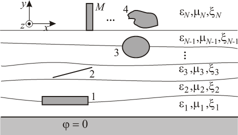
Fig. 1. Geometry of a multiconductor line in a layered bi-isotropic medium with zero potential plane.

The HBEM application for solving and analyzing bi-isotropic medium is described in detail in Section III. The electric and magnetic polarized surface charge distributions of a line charge placed above boundary surface of two bi-isotropic layers of Tellegen type is considered. These results will be compared with the analytical solution and used to verify the HBEM procedure. The next step is to analyze a microstrip with a ground plane of infinite width and a bi-isotropic substrate of finite width. Obtained HBEM results have been compared with results given by other researchers.

II CONSTITUTIVE RELATIONS FOR BI-ISOTROPIC MEDIUM

A bi-isotropic medium consists of elements with electric and magnetic dipoles. The constitutive relations for bi-isotropic materials are, [29],

$$\mathit{D}=\epsilon \mathit{E}+\xi \mathit{H}\mathrm{and}$$

(1)

$$\mathit{B}=\zeta \mathit{E}+\mu \mathit{H},$$

(2)

where $\xi$ and $\zeta$ are the magnetoelectric coupling coefficients, $\epsilon$ is the permittivity and $\mu$ is the permeability of medium. The parameters $\xi$ and $\zeta$ are usually given in the form

$$\zeta =(\chi +j\kappa )\sqrt{{\epsilon }_0{\mu }_0}\mathrm{and}$$

(3)

$$\xi =(\chi -j\kappa )\sqrt{{\epsilon }_0{\mu }_0}.$$

(4)

Replacing these parameters into eqns (1) and (2),

$$\mathit{D}=\epsilon \mathit{E}+(\chi -j\kappa )\sqrt{{\epsilon }_0{\mu }_0}\mathit{H}\mathrm{and}$$

(5)

$$\mathit{B}=(\chi +j\kappa )\sqrt{{\epsilon }_0{\mu }_0}\mathit{E}+\mu \mathit{H}.$$

(6)

Parameter $\kappa$ describes the degree of chirality, ${\epsilon }_0$ and ${\mu }_0$ are the permittivity and permeability of the air. Parameter $\chi$ is a dimensionless quantity for the degree of inherent nonreciprocity. Nonreciprocal nonchiral medium ($\chi \ne 0$, $\kappa =0$) is so-called Tellegen material, [29]. Such kind of media will be analyzed in this paper.

For Tellegen medium, it is satisfied $\zeta =\xi$, so the constitutive relations have the following form,

$$\mathit{D}=\epsilon \mathit{E}+\xi \mathit{H}\mathrm{and}$$

(7)

$$\mathit{B}=\xi \mathit{E}+\mu \mathit{H}.$$

(8)

The parameter $p={\xi }^2/(\epsilon \mu )$, $0<p<1$, describes the level of bi-isotropic effect, [18]. For example, if $p=0.1$, the media is with less expressed bi-isotropic effect. For $p=0.9$, the media has high level of bi-isotropy.

III HBEM APPLICATION

In order to apply the HBEM, the system given in Figure 2 is considered. A line charge $q^{\prime }$ is placed at height $h$ above the separating surface of two BI layers with parameters ${\epsilon }_1$, ${\mu }_1$, ${\xi }_1$ for the layer 1, and ${\epsilon }_2$, ${\mu }_2$, ${\xi }_2$ for the layer 2.

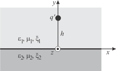
Fig. 2. Line charge placed above the boundary surface of two bi-isotropic layers.

The boundary surface between two BI layers of finite width $2L$ can be discretized as it is presented in Figure 3.

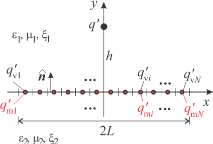
Fig. 3. HBEM application model.

The surface is divided into $N$ strips (segments) of width $\mathrm{\Delta }l=2L/N$. According to the HBEM application for the isotropic layers, [14], each of those segments should be replaced with equivalent electrodes (EEs) of radius $a_{\mathrm{e}}=\mathrm{\Delta }l/\pi$, placed along the segment’s axis. Those EEs are polarized line charges $q_{\mathrm{v}i}^{\prime }$ ($i=1,\mathrm{\hspace{0.17em}2},\mathrm{\dots },N$), placed in the air.

In order to apply HBEM for the BI layers, the necessary modification of the method includes an introduction of fictitious magnetic line charges $q_{\mathrm{m}i}^{\prime }$ ($i=1,\mathrm{\hspace{0.17em}2},\mathrm{\dots },N$). The positions and radii of these charges are the same as for the electric charges. Those charges are also placed in the air.

Based on the described procedure, a HBEM model, shown in Figure 3, is formed.

The electric and magnetic scalar potentials at any point $M(x,y)$ for the considered system given in Figure 3, are

$$\begin{array}{c}\hfill \phi =-\frac{q^{\prime }}{2\pi {\epsilon }_1(1-p_1)}\ln \sqrt{x^2+{(y-h)}^2}-\hfill \\ \hfill -\sum _{i=1}^N\frac{q_{\mathrm{v}i}^{\prime }}{2\pi {\epsilon }_0}\ln \sqrt{{(x-x_i)}^2+{(y-y_i)}^2},\hfill \end{array}$$

(9)

$$\begin{array}{c}\hfill {\phi }_{\mathrm{m}}=\frac{{\xi }_1{q}^{\prime }}{2\pi {\epsilon }_1{\mu }_1(1-p_1)}\ln \sqrt{x^2+{(y-h)}^2}-\hfill \\ \hfill -\sum _{i=1}^N\frac{q_{\mathrm{m}i}^{\prime }}{2\pi }\ln \sqrt{{(x-x_i)}^2+{(y-y_i)}^2},\hfill \end{array}$$

(10)

where $x_i=-L+(2i-1)\mathrm{\Delta }l/2$ and $y_i=0$ ($i=1,\mathrm{\hspace{0.17em}2},\mathrm{\dots },N$) are the line charges positions. The parameter $p_1$ is $p_1={\xi }_1^2/({\epsilon }_1{\mu }_1)$.

In order to determine the unknown values of the line charges, according to the HBEM procedure, [14], it is necessary to form a system of linear equations using the boundary condition, i.e. a relation between the normal component of the electric field and total surface charges. The HBEM application for BI materials needs a modification. It is necessary to use the relations between normal component of electric as well as magnetic field and total surface charges, i.e. electric and fictitious magnetic charges.

A Relations between normal components of electric as well as magnetic field at boundary surface of two BI media and total surface charges

Using eqns (7) and (8), the relations between the electromagnetic field components in the layer 1 and 2, for the system visible in the Figure 2 are, respectively,

$${\mathit{D}}_1={\epsilon }_1{\mathit{E}}_1+{\xi }_1{\mathit{H}}_1,$$

(11)

$${\mathit{D}}_2={\epsilon }_2{\mathit{E}}_2+{\xi }_2{\mathit{H}}_2,$$

(12)

$${\mathit{B}}_1={\mu }_1{\mathit{H}}_1+{\xi }_1{\mathit{E}}_1,$$

(13)

$${\mathit{B}}_2={\mu }_2{\mathit{H}}_2+{\xi }_2{\mathit{E}}_2.$$

(14)

Replacing those expressions into boundary conditions for the normal components of electric and magnetic fields, the following relations are obtained:

$${\epsilon }_1{E}_{1\mathrm{n}}+{\xi }_1{H}_{1\mathrm{n}}={\epsilon }_2{E}_{2\mathrm{n}}+{\xi }_2{H}_{2\mathrm{n}}\mathrm{and}$$

(15)

$${\mu }_1{H}_{1\mathrm{n}}+{\xi }_1{E}_{1\mathrm{n}}={\mu }_2{H}_{2\mathrm{n}}+{\xi }_2{E}_{2\mathrm{n}}.$$

(16)

From those equations, it can be written

$$E_{2\mathrm{n}}=\frac{{\epsilon }_1{\mu }_2-{\xi }_1{\xi }_2}{{\epsilon }_2{\mu }_2-{\xi }_2^2}{E}_{1\mathrm{n}}+\frac{{\xi }_1{\mu }_2-{\xi }_2{\mu }_1}{{\epsilon }_2{\mu }_2-{\xi }_2^2}{H}_{1\mathrm{n}},$$

(17)

$$H_{2\mathrm{n}}=\frac{{\xi }_1{\epsilon }_2-{\xi }_2{\epsilon }_1}{{\epsilon }_2{\mu }_2-{\xi }_2^2}{E}_{1\mathrm{n}}+\frac{{\epsilon }_2{\mu }_1-{\xi }_1{\xi }_2}{{\epsilon }_2{\mu }_2-{\xi }_2^2}{H}_{1\mathrm{n}}.$$

(18)

The electric polarized surface charge density, ${\eta }_v$, at the boundary surface between any two layers is, [18]

$${\eta }_v=P_{2\mathrm{n}}-P_{1\mathrm{n}},$$

(19)

where $P_{1\mathrm{n}}$ and $P_{2\mathrm{n}}$ are normal components of polarization vector in layers 1 and 2, respectively, defined as

$$P_{1\mathrm{n}}=({\epsilon }_1-{\epsilon }_0)E_{1\mathrm{n}}+{\xi }_1{H}_{1\mathrm{n}}\mathrm{and}$$

(20)

$$P_{2\mathrm{n}}=({\epsilon }_2-{\epsilon }_0)E_{2\mathrm{n}}+{\xi }_2{H}_{2\mathrm{n}}.$$

(21)

Replacing eqns. (17) and (18) into (21), the expression (19) is

${\eta }_v=$	${\displaystyle \frac{{\epsilon }_0[{\mu }_2({\epsilon }_2-{\epsilon }_1)-{\xi }_2^2+{\xi }_1{\xi }_2]}{{\epsilon }_2{\mu }_2-{\xi }_2^2}}{E}_{1\mathrm{n}}^{(0+)}+$	(22)
	$+{\displaystyle \frac{{\epsilon }_0[{\xi }_2{\mu }_1-{\xi }_1{\mu }_2]}{{\epsilon }_2{\mu }_2-{\xi }_2^2}}{H}_{1\mathrm{n}}^{(0+)}.$

The label (0+) indicates the electric and magnetic field components in layer 1 for $y=0$.

The magnetic polarized surface charge can be calculated as

$${\eta }_m=M_{2\mathrm{n}}-M_{1\mathrm{n}},$$

(23)

where the normal components of magnetization vector in layers 1 and 2, $M_{1\mathrm{n}}$ and $M_{2\mathrm{n}}$, are defined as

$$M_{1\mathrm{n}}=\left(\frac{{\mu }_1}{{\mu }_0}-1\right)H_{1\mathrm{n}}+\frac{{\xi }_1}{{\mu }_0}{E}_{1\mathrm{n}},$$

(24)

$$M_{2\mathrm{n}}=\left(\frac{{\mu }_2}{{\mu }_0}-1\right)H_{2\mathrm{n}}+\frac{{\xi }_2}{{\mu }_0}{E}_{2\mathrm{n}}.$$

(25)

Replacing eqns. (17) and (18) into (25), the expression (23) is

${\eta }_m=$	${\displaystyle \frac{{\xi }_2{\epsilon }_1-{\xi }_1{\epsilon }_2}{{\epsilon }_2{\mu }_2-{\xi }_2^2}}{E}_{1\mathrm{n}}^{(0+)}+$	(26)
	$+{\displaystyle \frac{{\epsilon }_2({\mu }_2-{\mu }_1)-{\xi }_2^2+{\xi }_1{\xi }_2}{{\epsilon }_2{\mu }_2-{\xi }_2^2}}{H}_{1\mathrm{n}}^{(0+)}.$

Using eqns (22) and (26), it is possible to express the relations between the normal components of electric as well as magnetic field and electric and magnetic polarized surface charges,

$$\widehat{n}{\mathit{E}}_{i0}^{(0+)}=\frac{{\epsilon }_2({\mu }_1-{\mu }_2)-{\xi }_1{\xi }_2+{\xi }_2^2}{{\epsilon }_0[({\epsilon }_1-{\epsilon }_2)({\mu }_2-{\mu }_1)+{({\xi }_1-{\xi }_2)}^2]}{\eta }_{\mathrm{v}i}+$$

$$+\frac{{\mu }_1{\xi }_2-{\mu }_2{\xi }_1}{({\epsilon }_1-{\epsilon }_2)({\mu }_2-{\mu }_1)+{({\xi }_1-{\xi }_2)}^2}{\eta }_{\mathrm{m}i},$$

(27)

$$\widehat{n}{\mathit{H}}_{i0}^{(0+)}=\frac{{\epsilon }_1{\xi }_2-{\epsilon }_2{\xi }_1}{{\epsilon }_0[({\epsilon }_1-{\epsilon }_2)({\mu }_2-{\mu }_1)+{({\xi }_1-{\xi }_2)}^2]}{\eta }_{\mathrm{v}i}+$$

$$+\frac{{\mu }_2({\epsilon }_1-{\epsilon }_2)-{\xi }_1{\xi }_2+{\xi }_2^2}{({\epsilon }_1-{\epsilon }_2)({\mu }_2-{\mu }_1)+{({\xi }_1-{\xi }_2)}^2}{\eta }_{\mathrm{m}i},$$

(28)

where ${\eta }_{\mathrm{v}i}=q_{\mathrm{v}i}^{\prime }/\mathrm{\Delta }l$ and ${\eta }_{\mathrm{m}i}=q_{\mathrm{m}i}^{\prime }/\mathrm{\Delta }l$ ($i=1,\mathrm{\hspace{0.17em}2},\mathrm{\dots },N$) are electric and magnetic polarized surface charges for $i-$th segment. $\widehat{n}=\widehat{y}$ is a unit normal vector. $q_{\mathrm{v}i}^{\prime }$ and $q_{\mathrm{m}i}^{\prime }$ expressed over the normal components of electric and magnetic fields are

$q_{\mathrm{v}i}^{\prime }=$	${\displaystyle \frac{{\epsilon }_0[{\mu }_2({\epsilon }_2-{\epsilon }_1)-{\xi }_2^2+{\xi }_1{\xi }_2]}{{\epsilon }_2{\mu }_2-{\xi }_2^2}}\mathrm{\Delta }l{E}_y^{(0+)}+$	(29)
	$+{\displaystyle \frac{{\epsilon }_0[{\xi }_2{\mu }_1-{\xi }_1{\mu }_2]}{{\epsilon }_2{\mu }_2-{\xi }_2^2}}\mathrm{\Delta }l{H}_y^{(0+)},$

$q_{\mathrm{m}i}^{\prime }=$	${\displaystyle \frac{{\xi }_2{\epsilon }_1-{\xi }_1{\epsilon }_2}{{\epsilon }_2{\mu }_2-{\xi }_2^2}}\mathrm{\Delta }l{E}_y^{(0+)}+$	(30)
	$+{\displaystyle \frac{{\epsilon }_2({\mu }_2-{\mu }_1)-{\xi }_2^2+{\xi }_1{\xi }_2}{{\epsilon }_2{\mu }_2-{\xi }_2^2}}\mathrm{\Delta }l{H}_y^{(0+)}.$

B System of linear equations formulation

Unlike the HBEM, applied for modeling configurations presented in [14-17], where the PMM is applied only on the surfaces of electric charges (only those charges exist at separating surfaces), here it is necessary to apply the PMM on the surface of $i$-th magnetic line charge as well as on $i$-th electric line charge. So, the total number of unknowns is $2N$ and the formed system of equations has a dimension $2N\times 2N$. During this method application, it should be taken into account:

• An influence of the charge itself (electric or magnetic), with matching points: $x_{\mathrm{p}}=x_i$, $y_{\mathrm{p}}=a_{\mathrm{e}}$;

• An influence of other charge which is placed at the same position (magnetic or electric), with the matching points: $x_{\mathrm{p}}=x_i$, $y_{\mathrm{p}}=a_{\mathrm{e}}$;

• Influences of all the other electric and magnetic line charges, with the matching points: $x_{\mathrm{p}}=x_i$, $y_{\mathrm{p}}=0$,

• An influence of primary line charge, with the matching points: $x_{\mathrm{p}}=x_i$, $y_{\mathrm{p}}=0$.

Application of this procedure using eqns (29) and (30), gives the system of linear equations:

$q_{\mathrm{v}i}^{\prime }=$	$\mathrm{A}\mathrm{\Delta }l[{\displaystyle \frac{q^{\prime }}{2\pi {\epsilon }_1(1-p_1)}}{\displaystyle \frac{-h}{x_i^2+h^2}}+{\displaystyle \frac{q_{v1}^{\prime }}{2\pi {\epsilon }_0}}\cdot 0+$	(31)
	$+{\displaystyle \frac{q_{\mathrm{v2}}^{\prime }}{2\pi {\epsilon }_0}}\cdot 0+\mathrm{\dots }+{\displaystyle \frac{q_{\mathrm{v}i}^{\prime }}{2\pi {\epsilon }_0}}{\displaystyle \frac{1}{a_{\mathrm{e}}}}+\mathrm{\dots }+{\displaystyle \frac{q_{\mathrm{v}N}^{\prime }}{2\pi {\epsilon }_0}}\cdot 0]+$
	$+\mathrm{B}\mathrm{\Delta }l[{\displaystyle \frac{{\xi }_1{q}^{\prime }}{2\pi {\epsilon }_1{\mu }_1(1-p_1)}}{\displaystyle \frac{h}{x_i^2+h^2}}+{\displaystyle \frac{q_{\mathrm{m1}}^{\prime }}{2\pi }}\cdot 0+$
	$+{\displaystyle \frac{q_{\mathrm{m2}}^{\prime }}{2\pi }}\cdot 0+\mathrm{\dots }+{\displaystyle \frac{q_{\mathrm{m}i}^{\prime }}{2\pi }}{\displaystyle \frac{1}{a_{\mathrm{e}}}}+\mathrm{\dots }+{\displaystyle \frac{q_{\mathrm{m}N}^{\prime }}{2\pi }}\cdot 0],$

$q_{\mathrm{m}i}^{\prime }=$	$\mathrm{C}\mathrm{\Delta }l[{\displaystyle \frac{q^{\prime }}{2\pi {\epsilon }_1(1-p_1)}}{\displaystyle \frac{-h}{x_i^2+h^2}}+{\displaystyle \frac{q_{v1}^{\prime }}{2\pi {\epsilon }_0}}\cdot 0+$	(32)
	$+{\displaystyle \frac{q_{\mathrm{v2}}^{\prime }}{2\pi {\epsilon }_0}}\cdot 0+\mathrm{\dots }+{\displaystyle \frac{q_{\mathrm{v}i}^{\prime }}{2\pi {\epsilon }_0}}{\displaystyle \frac{1}{a_{\mathrm{e}}}}+\mathrm{\dots }+{\displaystyle \frac{q_{\mathrm{v}N}^{\prime }}{2\pi {\epsilon }_0}}\cdot 0]+$
	$+\mathrm{D}\mathrm{\Delta }l[{\displaystyle \frac{{\xi }_1{q}^{\prime }}{2\pi {\epsilon }_1{\mu }_1(1-p_1)}}{\displaystyle \frac{h}{x_i^2+h^2}}+{\displaystyle \frac{q_{\mathrm{m1}}^{\prime }}{2\pi }}\cdot 0+$
	$+{\displaystyle \frac{q_{\mathrm{m2}}^{\prime }}{2\pi }}\cdot 0+\mathrm{\dots }+{\displaystyle \frac{q_{\mathrm{m}i}^{\prime }}{2\pi }}{\displaystyle \frac{1}{a_{\mathrm{e}}}}+\mathrm{\dots }+{\displaystyle \frac{q_{\mathrm{m}N}^{\prime }}{2\pi }}\cdot 0],$

for $i=1,\mathrm{\hspace{0.17em}2},\mathrm{\dots },N$.

The constants A, B, C, and D are

$$\mathrm{A}=\frac{{\epsilon }_0[{\mu }_2({\epsilon }_2-{\epsilon }_1)-{\xi }_2^2+{\xi }_1{\xi }_2]}{{\epsilon }_2{\mu }_2-{\xi }_2^2},$$

(33)

$$\mathrm{B}=\frac{{\epsilon }_0[{\xi }_2{\mu }_1-{\xi }_1{\mu }_2]}{{\epsilon }_2{\mu }_2-{\xi }_2^2},$$

(34)

$$\mathrm{C}=\frac{{\xi }_2{\epsilon }_1-{\xi }_1{\epsilon }_2}{{\epsilon }_2{\mu }_2-{\xi }_2^2}\mathrm{and}$$

(35)

$$\mathrm{D}=\frac{{\epsilon }_2({\mu }_2-{\mu }_1)-{\xi }_2^2+{\xi }_1{\xi }_2}{{\epsilon }_2{\mu }_2-{\xi }_2^2}.$$

(36)

The expressions (31) and (32), after normalizations $q_{\mathrm{v}i}^{\prime }\text{’}/q^{\prime }$, $q_{\mathrm{m}i}^{\prime }\sqrt{{\epsilon }_0{\mu }_0}/q^{\prime }$ and $x{}_i/h$, as well as using that $a_{\mathrm{e}}=\mathrm{\Delta }l/\pi =2L/\pi N$, have a form

	${\displaystyle \frac{q_{\mathrm{v}i}^{\prime }}{q^{\prime }}}\left(1-{\displaystyle \frac{\mathrm{A}}{{\epsilon }_{0}2}}\right)-{\displaystyle \frac{q_{\mathrm{m}i}^{\prime }\sqrt{{\epsilon }_0{\mu }_0}}{q^{\prime }}}{\displaystyle \frac{\mathrm{B}}{2\sqrt{{\epsilon }_0{\mu }_0}}}=$	(37)
	$=\left(-\mathrm{A}+\mathrm{B}{\displaystyle \frac{{\xi }_1}{{\mu }_1}}\right){\displaystyle \frac{\frac{L}{h}}{\pi {\epsilon }_1(1-p_1)N\left(1+{\left(\frac{x_i}{h}\right)}^2\right)}}$

$$\begin{array}{cc}& -\frac{q_{\mathrm{v}i}^{\prime }}{q^{\prime }}\frac{\mathrm{C}}{{\epsilon }_{0}2}+\frac{q_{\mathrm{m}i}^{\prime }\sqrt{{\epsilon }_0{\mu }_0}}{q^{\prime }}\frac{1}{\sqrt{{\epsilon }_0{\mu }_0}}\left(1-\frac{\mathrm{D}}{2}\right)=\hfill \\ & =\left(-\mathrm{C}+\mathrm{D}\frac{{\xi }_1}{{\mu }_1}\right)\frac{\frac{L}{h}}{\pi {\epsilon }_1(1-p_1)N\left(1+{\left(\frac{x_i}{h}\right)}^2\right)}\hfill \end{array},$$

(38)

$$i=1,\mathrm{\hspace{0.17em}2},\mathrm{\dots },N.$$

After solving this system using Mathematica, the electric and magnetic polarized line charges are calculated. Also, it is possible to determine the electric and magnetic polarized surface charges.

IV RESULTS AND DISCUSSION

The normalized electric and magnetic polarized surface charges distributions along the boundary surface between two bi-isotropic layers for the system presented in Figure 2 are shown in Figures 4–7. Different types of bi-isotropic materials are analyzed.

The values for ${\epsilon }_{r1}$, ${\mu }_{r1}$, $p_1$ as well as ${\epsilon }_{r2}$, ${\mu }_{r2}$, $p_2$ are denoted in the figures. The other parameters, necessary for the HBEM application, are:

$$L/h=20,{\xi }_1=\sqrt{p_1{\epsilon }_0{\mu }_0{\epsilon }_{r1}{\mu }_{r1}},$$

$${\xi }_2=\sqrt{p_2{\epsilon }_0{\mu }_0{\epsilon }_{r2}{\mu }_{r2}},{\epsilon }_0=8.85\cdot {10}^{-12}\mathrm{F}/\mathrm{m},$$

$${\mu }_0=4\pi \cdot {10}^{-7}\mathrm{H}/\mathrm{m}\mathrm{and}N=100.$$

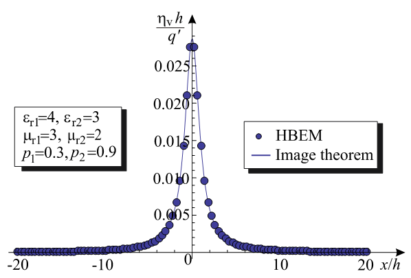
Fig. 4. Normalized electric polarized surface charges distribution on boundary surface of two layers with low and high bi-isotropic effects.

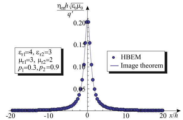
Fig. 5. Normalized magnetic polarized surface charges distribution on boundary surface of two layers with low and high bi-isotropic effects.

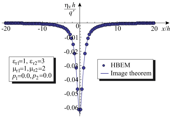
Fig. 6. Normalized electric polarized surface charges distribution on boundary surface of two isotropic layers.

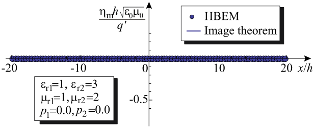
Fig. 7. Normalized magnetic polarized surface charges distribution on boundary surface of two isotropic layers.

In those figures, analytical solution results are also shown. These results have been calculated using eqns (22) and (26) as well as the expressions for the electric and magnetic fields in the bi-isotropic media, obtained using image theorem, [19].

The total number of unknown EEs for the HBEM calculation is $N_{tot}=2N=200$. The computation time is less than a second. Increasing the number of unknowns, the computation time increases too.

Analyzing the figures, where different types of BI effects are given, it can be concluded that the verification of HBEM procedure is successful. An excellent results match is obtained. So, there is no need for modification of used number of unknowns.

When both layers are isotropic, which is achieved for $p_1=p_2=0$, only electric polarized surface charges exists as it shown in Figures 6 and 7.

A Microstrip line with bi-isotropic substrate

According to the procedures described in Section III for bi-isotropic layers and in [15] for the isotropic media, a quasi-static analysis of microstrip line with a BI substrate of Tellegen type (Figure 8), is performed.

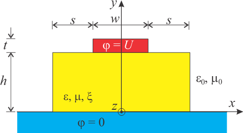
Fig. 8. Microstrip line with bi-isotropic substrate.

In order to form an equivalent HBEM model, it was necessary to apply the image theorem, considering that the substrate is placed on the zero potential plane of infinite width. That system is shown in Figure 9. With $q_{\mathrm{v}i}^{\prime }$, $q_{\mathrm{m}i}^{\prime }$ ($i=1,\mathrm{\dots },N$) and $q_{\mathrm{f}j}^{\prime }$ ($j=1,\mathrm{\dots },M$) are denoted polarized electric (v), fictitious magnetic (m) and free (f) line charges, respectively. All those charges are placed in the air, according to the HBEM.

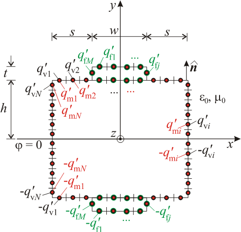
Fig. 9. HBEM application model.

The electric scalar as well as magnetic scalar potentials at any point of the system are:

$\phi =$	${\displaystyle \sum _{j=1}^M}{\displaystyle \frac{q_{\mathrm{f}j}^{\prime }}{2\pi {\epsilon }_0}}\ln \sqrt{{\displaystyle \frac{{(x-x_{\mathrm{f}j})}^2+{(y+y_{\mathrm{f}j})}^2}{{(x-x_{\mathrm{f}j})}^2+{(y-y_{\mathrm{f}j})}^2}}}+$	(39)
	$+{\displaystyle \sum _{i=1}^N}{\displaystyle \frac{q_{\mathrm{v}i}^{\prime }}{2\pi {\epsilon }_0}}\ln \sqrt{{\displaystyle \frac{{(x-x_{\mathrm{v}i})}^2+{(y+y_{\mathrm{v}i})}^2}{{(x-x_{\mathrm{v}i})}^2+{(y-y_{\mathrm{v}i})}^2}}},$

$${\phi }_{\mathrm{m}}=\sum _{i=1}^N\frac{q_{\mathrm{m}i}^{\prime }}{2\pi }\ln \sqrt{\frac{{(x-x_{\mathrm{m}i})}^2+{(y+y_{\mathrm{m}i})}^2}{{(x-x_{\mathrm{m}i})}^2+{(y-y_{\mathrm{m}i})}^2}}.$$

(40)

The total number of unknowns is $N_{\mathrm{tot}}=M+2N.$

Applying the procedure described in Section III, the unknown line charges are calculated, so the capacitance per unit length can be obtained using,

$$C^{\prime }=\sum _{j=1}^M\frac{q_{\mathrm{f}j}^{\prime }}{U}.$$

(41)

The characteristic impedance is determined as $Z_{\mathrm{c}}=Z_{\mathrm{c0}}\mathrm{/}\sqrt{{\epsilon }_{\mathrm{r}}^{\mathrm{eff}}}$, with ${\epsilon }_{\mathrm{r}}^{\mathrm{eff}}=C^{\prime }\mathrm{/}{C}_0^{\prime }$ the effective dielectric permittivity is denoted. $Z_{\mathrm{c0}}$ is the characteristic impedance of the stripline without dielectrics (free space). An optimal number of unknowns is determined according to the characteristic impedance results convergence, shown in Figure 10. In the same figure, with a dotted red line, the computation time for parameters: $h\mathrm{/}w=s\mathrm{/}w=1,$$t\mathrm{/}w=0.3$, ${\epsilon }_{\mathrm{r}}=3$, ${\mu }_{\mathrm{r}}=2$ and $p=0.2$, is also given.

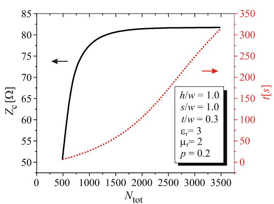
Fig. 10. Results convergence and computation time.

For all following calculations, the total number of unknowns will be $N_{tot}=1800.$

The results for characteristic impedance and effective relative permittivity have been compared with the results obtained using FlexPDE software, [30], in Table 1, for different values of parameter $p.$

Table 1: Characteristic impedance and effective relative permittivity values of microstrip line

	$Z_{\mathrm{c}}[\mathrm{\Omega }]$		${\epsilon }_r^{\mathrm{eff}}$
$p$	HBEM	FlexPDE	HBEM	FlexPDE
0	76.359	76.578	2.0890	2.0921
0.2	81.346	81.137	1.8410	1.8470
0.6	95.550	95.389	1.3341	1.3360
0.9	114.080	113.694	0.9360	0.9359

The microstrip dimensions and parameters are:

In this table, the values obtained for an isotropic substrate, for $p=0$, are also included. The characteristic parameters of a microstrip line with an isotropic substrate was analyzed separately in [15] and compared with available results. From Table 1, it can be concluded that a close results match is obtained. The error rate is less than 0.5%. The computation (CPU) time for both methods is given in Table 2. All calculations are performed on a quad-core CPU (Intel i5) running at 3.1 GHz and 4 GB RAM in double precision.

Table 2: CPU time

	Number of unknowns	Computation
		(CPU) time [s]
HBEM	1800 EEs	93
FlexPDE	151,162 finite elements	345

The CPU time in the HBEM application includes the time necessary to determine the positions of EEs, to fill the matrix, solve a formed system of linear equations as well as to calculate the characteristic parameters. On the other side, the FlexPDE CPU time consists of the time to run the problem, observe the output results, and calculate characteristic parameters.

The analysis of microstrip lines with a BI substrate is not so common in practice, as it is mentioned in the introduction of this paper. In [22], the characteristic impedance distribution of microstrip line with infinitely ground plane and BI substrate of Tellegen type is given. Those results as well as the results presented in [20] have been compared in Figure 11 with the HBEM results, for different values of relative permittivity and parameter $\chi$, where $\chi =\xi /\sqrt{{\epsilon }_0{\mu }_0}$.

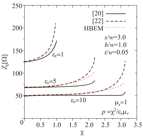
Fig. 11. Characteristic impedance as a function of parameter $\chi$ for different values of ${\epsilon }_r$.

The dimensions and parameters of analyzed microstrip line are: $h/w=1.0$, $s/w=3$, $t/w=0.05$, ${\mu }_r=1$, and $N=1800$.

In [22], it is mentioned that in [20] the authors made an assumption that electric charges do not create the magnetic flux, as well as the magnetic dipoles do not have any influence on the electric potential distribution. That is the main reason of large results disagreement in those two results, especially for larger values of parameter $\chi$. Significantly smaller disagreement can be noticed between HBEM results and those from [22]. It should be emphasized that HBEM analysis has been done for a configuration where the substrate has finite width and finite thickness, since in [20] and [22] the substrate has an infinite width as well as thickness.

V CONCLUSION

A development and implementation of HBEM, that started 10 years ago, have continued in this paper through the method extension for the analysis of BI media. It is now possible to analyze not only transmission lines, but also the other electromagnetic systems where BI materials are used. The HBEM’s application has been illustrated through the examples showing its generality and accuracy.

ACKNOWLEDGMENT

This work has been supported by the Ministry of Education, Science and Technological Development of the Republic of Serbia.

References

[1] D. M. Pozar, Microwave Engineering, John Wiley & Sons, New York, Chapter 1, pp. 2-6, 2012.

[2] M. Perić, Quasi-static approach for microwave transmission lines analysis, PhD thesis, Faculty of Electronic Engineering of Niš, Serbia, 2015. (in Serbian).

[3] T. Itoh and R. Mittra, “Analysis of microstrip transmission lines,” Advances in Microwaves, no. 8, pp. 67-141, 1974.

[4] E. Yamashita and R. Mittra, “Variational method for the analysis of microstrip lines,” IEEE Trans. Microwave Theory Tech., vol. 16, no. 4, pp. 251-256, Apr. 1968.

[5] T. Chang and C. Tan, “Analysis of a shielded microstrip line with finite metallization thickness by the boundary element method,” IEEE Trans. Microwave Theory Tech., no. 8, pp. 1130–1132, Aug. 1990.

[6] Z. Pantic and R. Mittra, “Quasi-TEM analysis of microwave transmission lines by the finite-element method,” IEEE Trans. Microwave Theory Tech., vol. 34, no. 11, pp. 1096–1103, Nov. 1986.

[7] Y. M. Tao, D. G. Fang, and X. G. Li, “Full-wave hybrid-mode analysis of general structure of coplanar waveguides by using the method of lines,” Microwave Opt. Technol. Lett., vol. 7, no. 1, pp. 17–19, Jan. 1994.

[8] N. Raičević, S. Aleksić, and S. Ilić, “A hybrid boundary element method for multi-layer electrostatic and magnetostatic problems,” Journal of Electromagnetics, vol. 30, no. 6, pp. 507-524, 2010.

[9] D. M. Veličković, “Equivalent electrodes method,” Scientific Review, no. 21-22, pp. 207-248, 1996.

[10] C. A. Brebbi, J. C. F. Telles, and L. C. Wrobel., Boundary Element Techniques: Theory and Applications in Engineering, Springer, Berlin, 1984.

[11] N. Raičević, S. Ilić, and S. Aleksić, “Application of new hybrid boundary element method on the cable terminations,” 14th International IGTE Symposium, Graz, Austria, pp. 56-61, Sept. 2010.

[12] A. Vučković, N. Raičević, and M. Perić, “Radially magnetized ring permanent magnet modelling in the vicinity of soft magnetic cylinder,” Safety Engineering, vol. 8, no. 1, pp. 33-37, 2018.

[13] A. Vučković, D. Vučković, M. Perić, and N. Raičević, “Influence of the magnetization vector misalignment on the magnetic force of permanent ring magnet and soft magnetic cylinder,” Int. Journal of Applied Electromagnetics and Mechanics, IOS Press, vol. 65, no. 3, pp. 417-430, 2021.

[14] S. Ilić, M. Perić, S. Aleksić, and N. Raičević, “Hybrid boundary element method and quasi TEM analysis of 2D transmission lines – generalization,” Electromagnetics, vol. 33, no. 4, pp. 292-310, Apr. 2013.

[15] M. Perić, S. Ilić, S. Aleksić, and N. Raičević, “Application of hybrid boundary element method to 2D microstrip lines analysis,” Int. Journal of Applied Electromagnetics and Mechanics, vol. 42, no. 2, pp. 179-190, 2013.

[16] M. Perić, S. Ilić, S. Aleksić, and N. Raičević, “Characteristic parameters determination of different striplines configurations using HBEM,” Applied Computational Electromagnetics Society (ACES) Journal, vol. 28, no. 9, pp. 858-865, Sept. 2013.

[17] M. Perić, S. Ilić, A. Vučković, and N. Raičević, “Improving the efficiency of hybrid boundary element method for electrostatic problems solving,” Applied Computational Electromagnetics Society (ACES) Journal, vol. 35, no. 8, pp. 872-877, Aug. 2020.

[18] E. Rothwell and M. Cloud, Electromagnetics, Chapter 2, CRC Press, 2001.

[19] D. M. Veličković and Ž. J. Mančić, “Low frequency electromagnetic field analysis in bianisotropic media,” 3${}^{r\mathit{}d}$ IEEE INTERMAG 93, Stockholm, Sweden, pp. 11-14, Apr. 1993.

[20] P. Koivisto and J. Sten, “Quasi-static image method applied to bi-isotropic microstrip geometry,” IEEE Trans. Microwave Theory Tech., vol. 43, no. 1, pp. 169–175, Jan. 1995.

[21] F. Olyslager, E. Laermans, and D. De Zutter, “Rigorous quasi-TEM analysis of multiconductor transmission lines in bi-isotropic media – part I: theoretical analysis for general inhomogeneous media and generalization to bianisotropic media,” IEEE Trans. Microwave Theory Tech., vol. 43, no. 7, pp. 1409-1415, July 1995.

[22] F. Olyslager, E. Laermans, and D. De Zutter, “Rigorous quasi-TEM analysis of multiconductor transmission lines in bi-isotropic media – part II: numerical solution for layered media,” IEEE Trans. Microwave Theory Tech., vol. 43, no. 7, pp. 1416-1423, July 1995.

[23] Ž. J. Mančić and V. V. Petrović, “Quasi-static analysis of the shielded microstrip line with bi-isotropic substrate by the strong FEM formulation,” 11${}^{t\mathit{}h}$ Int. Conference on Telecommunications in Modern Satellite, Cable and Broadcasting Services – TELSIKS 2013, Serbia, Niš, pp. 513-516, Oct. 2013.

[24] C. Zebiri, D. Sayad, S. Daudi, and F. Benabdelaziz, “Microstrip line printed on a bianisotropic medium,” Icosipe 2015, Algeria, Tlemcen, pp. 111-120, 2015.

[25] S. Daoudi, F. Benabdelaziz, C. Zebiri, and D. Sayad, “Generalized exponential matrix technique application for the evaluation of the dispersion characteristics of a chiro-ferrite shielded multilayered microstrip line,” Progress in Electromagnetic Research - PIER, vol. 61, pp. 1-14, 2017.

[26] A. Semichaevsky, A. Akyurtlu, D. Kern, and D. Werner, “Analysis of the interaction of electromagnetic waves with a chyral cylinder using a novel FDTD approach,” 20${}^{t\mathit{}h}$ Annual Review of Progress in Applied Computational Electromagnetics Society (ACES), USA, April 19-23, 2004.

[27] S. T. Imeci, F. Altunkilic, J. R. Mautz, and E. Arvas, “Transmission through an arbitrarily shaped aperture in a conducting plane separating air and a chiral medium,” Applied Computational Electromagnetics Society (ACES) Journal, vol. 25, no. 7, pp. 587-599, July 2010.

[28] A. B. Olcen, S. T. Imeci, M. Gokten, J. Mautz, and E. Arvas, “Method of moments analysis of electromagnetic transmission though an arbitrarily shaped 3D cavity in a thick conducting plane,” Applied Computational Electromagnetics Society (ACES) Journal, vol. 30, no. 11, pp. 1137-1145, Nov. 2015.

[29] A. H. Sihvola, “Electromagnetic modeling of bi-isotropic media,” Progress in Electromagnetic Research - PIER, no. 9, pp. 45-86, 1994.

[30] FlexPDE, ver. 5, PDE Solutions Inc., 2009.

Biographies

Mirjana Perić received the Dipl.–Ing., M.Sc. and Ph.D. degrees from the Faculty of Electronic Engineering (FEE) of Niš, Serbia. In 2001, she joined the Department of Theoretical Electrical Engineering at the FEE. She is currently an assistant professor at the same faculty.

Her researching interests are: electromagnetic field theory, analytical and numerical methods for electromagnetic field calculations, electromagnetic compatibility, and transmission line analysis.

She is a member of the ACES, IEEE MTT and IEEE EMC societies.

Saša S. Ilić received Dipl.-Ing. degree in electronics and telecommunications in 1995 from the Faculty of Electronic Engineering (FEE) of Niš, Serbia. At the same faculty he received M.Sc. and Ph.D. degrees in theoretical electrical engineering in 2001 and 2014, respectively.

From January 1998 up to now, he has engaged to the Department of Theoretical Electrical Engineering, at the FEE.

His researching areas are: lightning protection systems, low-frequency electromagnetic fields penetrated into human body and microstrip transmission lines analysis with isotropic, anisotropic, and bianisotropic media.

Ana Vučković received the Dipl.-Ing., M.Sc., and Ph.D. degrees from the Faculty of Electronic Engineering of Niš, Serbia. In 2003, she joined the Department of Theoretical Electrical Engineering at the FEE. She works as an assistant professor at the same faculty.

Her main research area is computational electromagnetics (electromagnetic field theory, analytical and numerical methods for electromagnetic field calculations, electromagnetic compatibility and permanent magnet analysis). Also, she took part in numerous international projects and projects supported by the Serbian Ministry of Education and Science. She is a member of the ACES society.

Nebojša Raičević received his Dipl.-Ing., M. Sc., and Ph.D. degrees at the Faculty of Electronic Engineering (FEE) of Niš, Serbia, in 1989, 1998, and 2010, respectively. He received the Dr.-Ing. degree with a PhD-thesis dealing with the numerical electromagnetic field calculations.

He is currently an associate professor at the FEE. His research interests include: cable terminations and joints, numerical methods for EM problems solving, microstrip transmission lines with isotropic, anisotropic, and bianisotropic media, metamaterial structures, EMC, nonlinear electrostatic problems, magnetic field calculation of coils and permanent magnets. He is a member of the IEEE AP Society, IEEE EMC Society, IEEE Dielectrics and Electrical Insulation Society, and IEEE Magnetics Society.

ACES JOURNAL, Vol. 36, No. 10, 1265–1273.
doi: 10.13052/2021.ACES.J.361001
© 2021 River Publishers

Abstract

I INTRODUCTION

II CONSTITUTIVE RELATIONS FOR BI-ISOTROPIC MEDIUM

III HBEM APPLICATION

A Relations between normal components of electric as well as magnetic field at boundary surface of two BI media and total surface charges

B System of linear equations formulation

IV RESULTS AND DISCUSSION

A Microstrip line with bi-isotropic substrate

V CONCLUSION

ACKNOWLEDGMENT

References

Biographies