Efficient Method Based on SMW Formula for Analyzing PEC Targets with Partial and Thin Coatings

Zhiwen Dong¹, Xinlei Chen^{1, 2, 3}, Guiyue Yu¹, Ziwei Li¹, Lichang Lu¹, and Changqing Gu¹

¹Key Laboratory of Radar Imaging and Microwave Photonics, College of Electronic and Information Engineering, Nanjing University of Aeronautics and Astronautics, Nanjing, China

²Key Laboratory of Meteorological Disaster (KLME) Ministry of Education & Collaborative Innovation Center on Forecast and Evaluation of Meteorological Disasters (CIC-FEMD), Nanjing University of Information Science & Technology, Nanjing, China

³State Key Laboratory of Millimeter Waves, Southeast University, China

dongzw@nuaa.edu.cn, chenxl@nuaa.edu.cn, yuguiyue@nuaa.edu.cn, liziwei@nuaa.edu.cn, llchang@nuaa.edu.cn, gucq@nuaa.edu.cn

Submitted On: May 9, 2021; Accepted On: September 9, 2021

Abstract

The analysis of the electromagnetic scattering from the perfect electric conductor (PEC) partially coated with thin material is a significant task in stealth design. Previous research has shown the scattering can be calculated by only discretizing the current on PEC in the case of thin coating layers. However, it has a downside that it will recalculate a complete solution when the geometry or electromagnetic properties of the coating changes. In this paper, a Sherman–Morrison–Woodbury (SMW) formula-based method is proposed to address this problem. According to the SMW formulation, it can reuse the inverse impedance matrix of the PEC part to efficiently obtain the solutions when local coating changes, so it can avoid the subsequent complete inverse of the new impedance matrix. Furthermore, it employs the fast direct solution method based on the SMW formulation to accelerate the calculation of inverse matrix of the PEC part. Numerical results demonstrate the performance of the proposed method.

Index Terms: electromagnetic scattering, method of moments, Sherman–Morrison–Woodbury formula, thin coating.

I INTRODUCTION

It is a significant task to calculate the radar cross section (RCS) of a target accurately and efficiently, especially for the perfect electric conductor (PEC) coated by material layers, cause of its wide application in stealth design. In the context of MoM [1], the surface integral equation (SIE) [2] and the volume surface integral equation (VSIE) [3] are usual ways to solve the type of problem. According to the equivalence principle, the SIE will induce the electric current and the magnetic current on the interface between different materials. The VSIE will discrete the material part into tetrahedral meshes.

For analyzing the scattering of PEC coated by thin material layer, the thin dielectric sheet (TDS) [4], [5] method can be employed. It requires less basis functions and is more efficient than the conventional SIE and VSIE [4], [5], however, it still employs extra basis functions to expand the electric current within material layers, compared with calculating the PEC without coating. Recently, another way to solve the thin coating problem is regarding the polarization sources as constant and using the surface current on the PEC to express them [6], [7]. As a result, no additional basis functions are needed compared to analyze the scattering of PEC without coating.

Nevertheless, a problem in the approach [6], [7] is the repetitive computation of impedance matrix and the LU decomposition when analyzing the scattering of the PEC with different local coating situations, which results in intensely expensive CPU time just for the same PEC model. In this paper, a scheme based on the Sherman–Morrison–Woodbury (SMW) formula [8]-[11] is proposed to address this problem. It divides the total impedance matrix into two parts. One is the PEC matrix which is the invariable part. The other one is the polarization part that is varying in each coating situation. In accordance with SMW formula [8]-[11], the inverse of impedance matrix is transformed to another form containing the inverse of the unchanged PEC matrix. The inverse of the PEC matrix only needs to be calculated once and can be reused for different coatings. No recalculation of the complete impedance matrix and another LU decomposition are needed in different local coating schemes. Furthermore, in order to further enhance the computational efficiency, the fast direct solver [12]-[14] based on the SMW formula, termed the SMW algorithm (SMWA) in [12], is applied to accelerate the inverse of the PEC matrix.

II FORMULATION

A Conventional method for PEC with thin coating

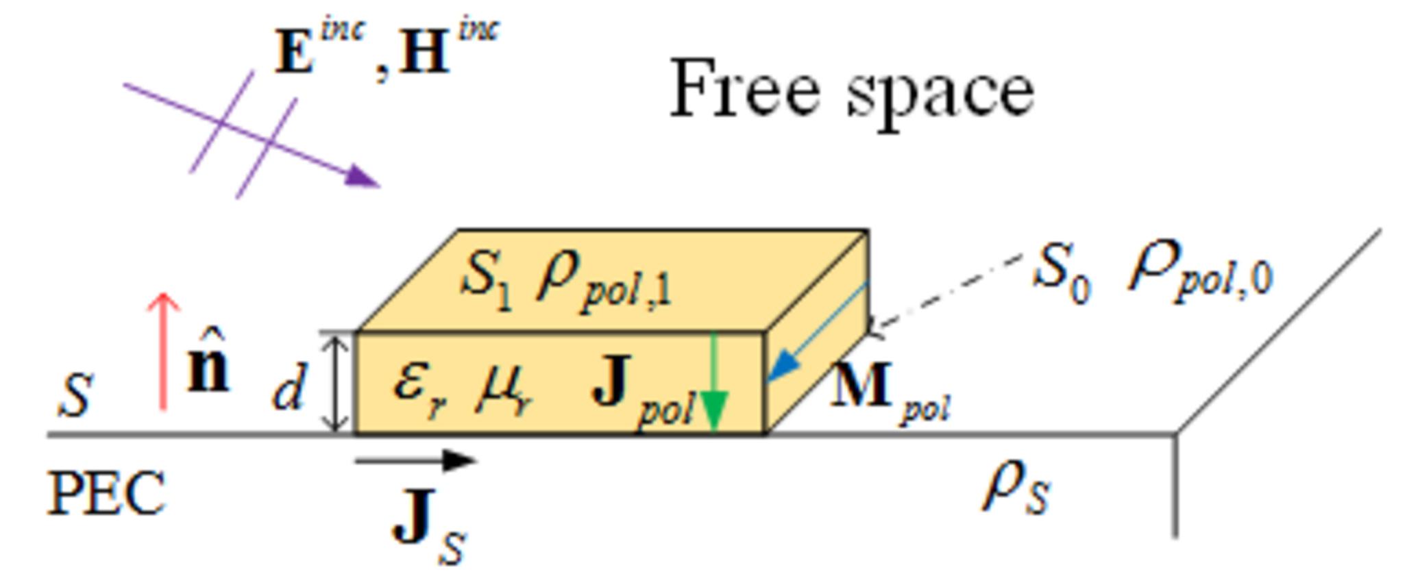
Fig. 1. A PEC partially coated with thin material. $S_0$ is the interface between the conductor and thin material. $S_1$ is the interface between the free space and thin material.

A PEC partially coated by thin material is illuminated by an incident plane wave $(E^{inc},H^{inc})$, as shown in Figure 1. The relative permittivity, relative permeability, and thickness of the material layer are ${\epsilon }_r$, ${\mu }_r$ and $d$, respectively. The scattering electric field can be expressed through the source induced by the plane wave. There are five forms of the source: surface electric current $J_s$ and surface charges ${\rho }_s$ on the conductor, polarization surface charges ${\rho }_{pol,0}$ on the interface $S_0$ between the conductor and the material, polarization surface charges ${\rho }_{pol,1}$ on the interface $S_1$ between the material and the free space, and polarization volume electric current $J_{pol}$ and polarization volume magnetic current $M_{pol}$ within the material layer. According to the relation between the field and the source, the electric field integral equation (EFIE) on the surface of the PEC can be expressed as [6], [7]

$$\begin{array}{c}{{\mathbf{E}}^{inc}|}_t=-{{\mathbf{E}}^{sca}|}_t\hfill \\ =[j\omega {\mu }_0{\int }_S{\mathbf{J}}_s\left({\mathbf{r}}^{\prime }\right)G\mathrm{d}{s}^{\prime }+\frac{1}{{\epsilon }_0}{\int }_S{\rho }_s\left({\mathbf{r}}^{\prime }\right)\nabla G\mathrm{d}{s}^{\prime }\hfill \\ +j\omega {\mu }_0{\int }_V{\mathbf{J}}_{pol}\left({\mathbf{r}}^{\prime }\right)Gd{v}^{\prime }+\frac{1}{{\epsilon }_0}{\int }_{S_0}{\rho }_{pol,0}\left({\mathbf{r}}^{\prime }\right)\nabla G\mathrm{d}{s}^{\prime }\hfill \\ +\frac{1}{{\epsilon }_0}{\int }_{S_1}{\rho }_{pol,1}\left({\mathbf{r}}^{\prime }\right)\nabla G\mathrm{d}{s}^{\prime }+{\int }_V\nabla G\times {\mathbf{M}}_{pol}\left({\mathbf{r}}^{\prime }\right)\mathrm{d}{v}^{\prime }]{}_t\hfill \end{array},$$

(1)

where $G(\mathbf{r},{\mathbf{r}}^{\prime })$ is the scalar Green’s function in free space. The integral domain V means the volume of thin material.

When the thickness of material layer is very thin relative to wavelength in material, only normal component of the polarization volume electric current and tangential component of the polarization volume magnetic current in the layer can be remained and regarded as constants [6], [7]. Then, the volume integrals can be transformed into surface integrals written as follows

$$\begin{array}{c}\hfill {\mathbf{E}}^{inc}{|}_t=[j\omega {\mu }_0{\int }_S{\mathbf{J}}_s\left({\mathbf{r}}^{\prime }\right)G\text{d}{s}^{\prime }+\frac{1}{{\epsilon }_0}{\int }_S{\rho }_s\left({\mathbf{r}}^{\prime }\right)\nabla G\text{d}{s}^{\prime }\hfill \\ \hfill +j\omega {\mu }_{0}d{\int }_{S_m}{\mathbf{J}}_{pol}\left({\mathbf{r}}^{\prime }\right)G\text{d}{s}^{\prime }+\frac{1}{{\epsilon }_0}{\int }_{S_0}{\rho }_{pol,0}\left({\mathbf{r}}^{\prime }\right)\nabla G\text{d}{s}^{\prime }\hfill \\ \hfill +\frac{1}{{\epsilon }_0}{\int }_{S_1}{\rho }_{pol,1}\left({\mathbf{r}}^{\prime }\right)\nabla G\text{d}{s}^{\prime }+d{\int }_{S_m}\nabla G\times {\mathbf{M}}_{pol}\left({\mathbf{r}}^{\prime }\right)\text{d}{s}^{\prime }]{}_t\hfill \end{array},$$

(2)

by using the relation $\mathrm{d}{v}^{\prime }=d\times \mathrm{d}{s}^{\prime }$. $S_m$ represents the middle surface of layer V.

The charges ${\rho }_s$ on the conductor can be obtained by the electric current continuity equation

$$-j\omega {\rho }_s={\nabla }_s\cdot {\mathbf{J}}_s.$$

(3)

The polarization volume electric current and the polarization volume magnetic current in material can be expressed by the electric field and the magnetic field [6], [7]

${\mathbf{J}}_{pol}$	$=j\omega {\epsilon }_0\left({\epsilon }_r-1\right)\mathbf{E},$	(4)
${\mathbf{M}}_{pol}$	$=j\omega {\mu }_0\left({\mu }_r-1\right)\mathbf{H}.$	(5)

According to the boundary condition on PEC surface

$$\widehat{\mathbf{n}}\cdot \mathbf{D}={\rho }_s,$$	(6)
$$\widehat{\mathbf{n}}\times \mathbf{H}={\mathbf{J}}_s,$$	(7)

where $\widehat{\mathbf{n}}$ is the unit normal vector from the inside to the outside of the PEC part, as shown in Figure 1. And with the help of the relation

$$\mathbf{D}=\epsilon \mathbf{E},$$	(8)
$$-\mathbf{H}=\widehat{\mathbf{n}}\times \left(\widehat{\mathbf{n}}\times \mathbf{H}\right),$$	(9)

we can get the relations

$$\widehat{\mathbf{n}}\cdot \epsilon \mathbf{E}={\rho }_s,$$	(10)
$$\mathbf{H}=-\widehat{\mathbf{n}}\times {\mathbf{J}}_s.$$	(11)

Substituting (10) and (11) into (4) and (5), and according to (3), the polarization volume electric current and the polarization volume magnetic current within the material layer can be represented by the surface current $J_s$ on PEC [6], [7].

$${\mathbf{J}}_{pol}=-\frac{{\epsilon }_r-1}{{\epsilon }_r}\left(\nabla \cdot {\mathbf{J}}_s\right)\widehat{\mathbf{n}},$$	(12)
$${\mathbf{M}}_{pol}=-j\omega {\mu }_0\left({\mu }_r-1\right)\widehat{\mathbf{n}}\times {\mathbf{J}}_s.$$	(13)

As to the polarization surface charges ${\rho }_{pol,i}$, the expression can derive from the boundary situation that the polarization charges can only remain in the material, here expressed as [6]

$$-j\omega {\rho }_{pol,0}=\widehat{\mathbf{n}}\cdot \left({\mathbf{J}}_{pol}-\mathbf{0}\right),$$	(14)
$$-j\omega {\rho }_{pol,1}=\widehat{\mathbf{n}}\cdot \left(\mathbf{0}-{\mathbf{J}}_{pol}\right),$$	(15)

because of no polarization volume current existing in conductor or free space. The polarization surface charge ${\rho }_{pol,i}$ can be eventually expressed as [6]

$${\rho }_{pol,0}=-{\rho }_{pol,1}=\frac{1}{j\omega }\cdot \frac{{\epsilon }_r-1}{{\epsilon }_r}\nabla \cdot {\mathbf{J}}_s.$$

(16)

Substituting (3), (12), (13), (16) into (2), we can find that the only unknown is ${\mathbf{J}}_s$ and the number of unknowns for this model is equal to that of unknowns required only for PEC surface of this model. No additional basis functions are needed, and no additional memory storage is required.

By applying the MoM [1], (2) can be converted into the matrix equation

$${\mathbf{Z}}^t\mathbf{I}={\mathbf{V}}^i,$$

(17)

where the elements of $Z^t$ and $V^i$ are

$$\begin{array}{c}\hfill Z_{mn}^t=j\omega {\mu }_0{\int }_{T_m}{\int }_{T_n}\left({\mathbf{f}}_m\cdot {\mathbf{f}}_n-\frac{1}{k_0^2}\nabla \cdot {\mathbf{f}}_m{\nabla }^{\prime }\cdot {\mathbf{f}}_n\right)G\text{d}{s}^{\prime }\text{d}s\hfill \\ \hfill -j\omega {\mu }_0\frac{{\epsilon }_r-1}{{\epsilon }_r}d{\int }_{T_m}{\int }_{T_n^{S_m}}{\mathbf{f}}_m\cdot \left[{\nabla }^{\prime }\cdot {\mathbf{f}}_n\right]\widehat{\mathbf{n}}\left({\mathbf{r}}^{\prime }\right)G\text{d}{s}^{\prime }\text{d}s\hfill \\ \hfill +\frac{1}{j\omega {\epsilon }_0}\frac{{\epsilon }_r-1}{{\epsilon }_r}{\int }_{T_m}{\int }_{T_n}{\mathbf{f}}_m\cdot \left[{\nabla }^{\prime }\cdot {\mathbf{f}}_n\right]\nabla G\text{d}{s}^{\prime }\text{d}s\hfill \\ \hfill -\frac{1}{j\omega {\epsilon }_0}\frac{{\epsilon }_r-1}{{\epsilon }_r}{\int }_{T_m}{\int }_{T_n^{S_1}}{\mathbf{f}}_m\cdot \left[{\nabla }^{\prime }\cdot {\mathbf{f}}_n\right]\nabla G\text{d}{s}^{\prime }\text{d}s\hfill \\ \hfill +j\omega {\mu }_0\left({\mu }_r-1\right)d{\int }_{T_m}{\int }_{T_n^{S_m}}{\mathbf{f}}_m\cdot \left[\widehat{\mathbf{n}}\left({\mathbf{r}}^{\prime }\right)\times {\mathbf{f}}_n\times \nabla G\right]\text{d}{s}^{\prime }\text{d}s\hfill \end{array},$$

(18)

$$V_m^i={\int }_{T_m}{\mathbf{f}}_m\cdot {\mathbf{E}}^{inc}\text{d}s,$$

(19)

${\mathbf{f}}_m$ and ${\mathbf{f}}_n$ stand for the mth test Rao–Wilton–Glisson (RWG) function [17] and the nth RWG basis function, respectively. The integral domain $T_n^{S_1}$ and $T_n^{S_m}$ in (18) represent $T_n$ shifted along the normal vector $\widehat{\mathbf{n}}$ to surface $S_1$ and $S_m$, respectively.

B Efficient method for PEC with partial and thin coating

Only the same conductor partially covered by different thin material is considered in this paper. For the conventional method, if either the electromagnetic properties of local coating or its geometry such as area, position, or thickness changes several times, ${\mathbf{Z}}^t$ and its LU decomposition need to be calculated repeatedly when the metal part of the model remains in its original form. The conventional method is expensive for this situation. In this section, an efficient method based on the SMW formula [8]-[11] is proposed to address this problem.

It can be seen from (18) that the element $Z_{mn}^t$ consists of two parts, PEC part $Z_{mn}$ and polarization part $P_{mn}^t$

$$Z_{mn}^t=Z_{mn}+P_{mn}^t,$$

(20)

where the element $Z_{mn}$ of the PEC impedance matrix Z and $P_{mn}^t$ of the polarization impedance matrix ${\mathbf{P}}^t$ are

$$Z_{mn}=j\omega {\mu }_0{\int }_{T_m}{\int }_{T_n}\left({\mathbf{f}}_m\cdot {\mathbf{f}}_n-\frac{1}{k_0^2}\nabla \cdot {\mathbf{f}}_m{\nabla }^{\prime }\cdot {\mathbf{f}}_n\right)G\text{d}{s}^{\prime }\text{d}s,$$

(21)

$$\begin{array}{c}\hfill P_{mn}^t=-j\omega {\mu }_0\frac{{\epsilon }_r-1}{{\epsilon }_r}d{\int }_{T_m}{\int }_{T_n^{S_m}}{\mathbf{f}}_m\cdot \left[{\nabla }^{\prime }\cdot {\mathbf{f}}_n\right]\widehat{\mathbf{n}}\left({\mathbf{r}}^{\prime }\right)G\text{d}{s}^{\prime }\text{d}s\hfill \\ \hfill +\frac{1}{j\omega {\epsilon }_0}\frac{{\epsilon }_r-1}{{\epsilon }_r}{\int }_{T_m}{\int }_{T_n}{\mathbf{f}}_m\cdot \left[{\nabla }^{\prime }\cdot {\mathbf{f}}_n\right]\nabla G\text{d}{s}^{\prime }\text{d}s\hfill \\ \hfill -\frac{1}{j\omega {\epsilon }_0}\frac{{\epsilon }_r-1}{{\epsilon }_r}{\int }_{T_m}{\int }_{T_n^{S_1}}{\mathbf{f}}_m\cdot \left[{\nabla }^{\prime }\cdot {\mathbf{f}}_n\right]\nabla G\text{d}{s}^{\prime }\text{d}s\hfill \\ \hfill +j\omega {\mu }_0\left({\mu }_r-1\right)d{\int }_{T_m}{\int }_{T_n^{S_m}}{\mathbf{f}}_m\cdot \left[\widehat{\mathbf{n}}\left({\mathbf{r}}^{\prime }\right)\times {\mathbf{f}}_n\times \nabla G\right]\text{d}{s}^{\prime }\text{d}s\hfill \end{array},$$

(22)

It suggests that for the same conductor the PEC matrix Z is unchanged and can be reused for different coatings. If somewhere on a metal surface is not covered by coatings, the corresponding polarization element $P_{mn}^t$ is zero and the corresponding column of the polarization matrix ${\mathbf{\text{P}}}^t$ is zero, as shown in Figure 2.

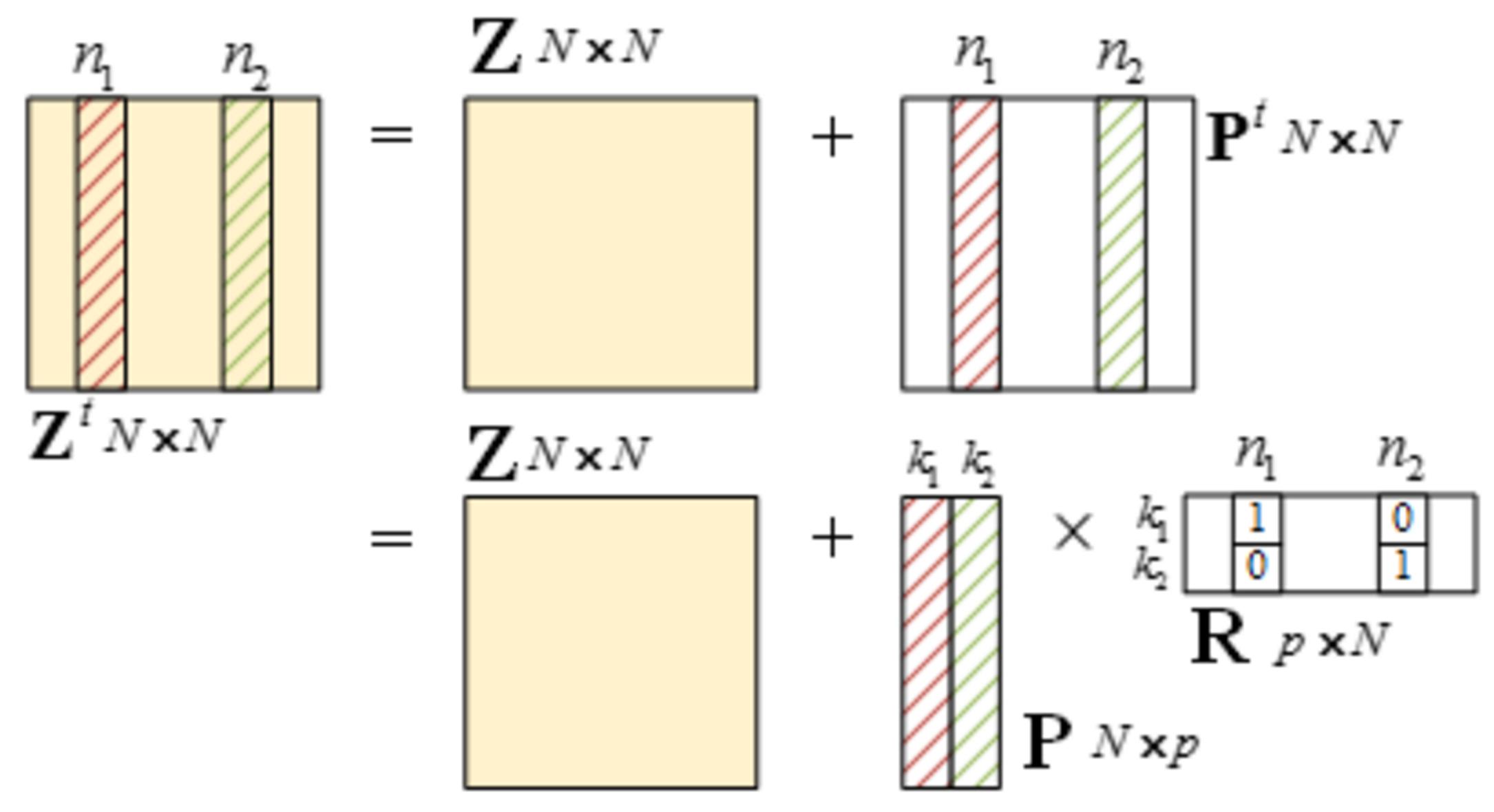
Fig. 2. The total impedance matrix $Z^t$ is divided into two parts.

The polarization matrix ${\mathbf{\text{P}}}^t$ can be further expressed as a product of two matrices, so (17) can be rewritten as

$${\mathbf{Z}}^t\mathbf{I}=\left(\mathbf{Z}+{\mathbf{P}}^t\right)\mathbf{I}=\left(\mathbf{Z}+\mathbf{PR}\right)\mathbf{I}\text{ = }{\mathbf{V}}^i,$$

(23)

where P is the impedance matrix of the polarization part, and R is the matrix consisting of 0 and 1. The matrix element $P_{mk}$ is the same as the element $P_{mn}^t$, which means if the $n_l$th column of ${\mathbf{\text{P}}}^t$ is at the $k_l$th column of matrix P, then the expression of matrix R is

$$R_{ij}=\{\begin{array}{c}\hfill 1\hfill \\ \hfill 0\hfill \end{array}\begin{array}{c}\end{array}\begin{array}{c}\end{array}\begin{array}{c}\hfill i=k_l,j=n_l\hfill \\ \hfill else\hfill \end{array}.$$

(24)

Assuming that the number of columns in P is p, the number of rows in R is also p, where p is the number of the basis function covered by material. The number of rows in P and the number of columns in R still are N. N is the total number of basis functions. In situation of local coating, p is very small compared to N. A simple example is shown in Figure 2 with p = 2.

With the change of coating geometry or coating properties, Z remains unchanged while P and R change. Utilizing the SMW formula [8]-[11], the current coefficient matrix I can be deduced

$\mathbf{I}$	$=\left(\mathbf{Z}+\mathbf{PR}\right){}^{-1}\mathbf{V}^i$	(25)
	$=\left({\mathbf{Z}}^{-1}{\mathbf{V}}^i\right)-\left({\mathbf{Z}}^{-1}\mathbf{P}\right){\left[\mathbf{1}+\mathbf{R}\left({\mathbf{Z}}^{-1}\mathbf{P}\right)\right]}^{-1}\mathbf{R}\left({\mathbf{Z}}^{-1}{\mathbf{V}}^i\right),$

where 1 represents the identity matrix. The LU decomposition of Z only needs to be computed once. The size of $\mathbf{1}+{\mathbf{RZ}}^{-1}\mathbf{P}$ is p, which is much smaller than the size of Z of N, so it takes less time to compute the LU decomposition of $\mathbf{1}+{\mathbf{RZ}}^{-1}\mathbf{P}$ than the LU decomposition of ${\mathbf{Z}}^t$ . For the analysis of a variety of different coating material, the inverse of PEC matrix can be reused rather than recalculating the inverse of a new matrix. As the number of changes increases, this method is more efficient than the conventional method.

In (25), the matrix equation needs to be solved

$${\mathbf{Z}}^{-1}\mathbf{B},$$

(26)

where $\mathbf{B}$ denotes ${\mathbf{V}}^i$ or $\mathbf{P}$. Although the inverse of Z only needs to be computed once, it is still expensive to calculate the inverse of Z when the unknowns increase. To address this problem, the SMWA [12]-[14], which is also based on the SMW formula, is used to efficiently solve (26). In the SMWA, a binary tree is used to divide the impedance matrix Z into different blocks in order to avoid calculating the inverse of the complete matrix Z and instead calculate the inverse of small blocks. The matrix after the partitioning of the one-level binary tree is shown as

$$Z=\left[\begin{array}{ll}{}^1{Z}_{11}\hfill & {}^1{Z}_{12}\hfill \\ {}^1{Z}_{21}\hfill & {}^1{Z}_{22}\hfill \end{array}\right],$$

(27)

where ${}^1\mathbf{Z}_{11}$ and ${}^1\mathbf{Z}_{22}$ are the self-impedance matrices of block 1 and 2 in matrix Z, respectively, while ${}^1\mathbf{Z}_{12}$ and ${}^1\mathbf{Z}_{21}$ are the mutual-impedance matrices between block 1 and 2 in matrix Z. The initial matrix Z can be represented as the product of a block diagonal matrix only containing self-impedance blocks ${}^q\mathbf{Z}_d$ and a special form matrix ${\mathbf{Z}}_q$containing identity matrix block and mutual-impedance blocks updated by self-impedance block expressed as

$$Z{=}^1{Z}_d{Z}_1=\left[\begin{array}{cc}{}^1{Z}_{11}& 0\\ 0& {}^1{Z}_{22}\end{array}\right]\left[\begin{array}{cc}1& {}^1{Z}_{11}^{-11}{Z}_{12}\\ {}^1{Z}_{22}^{-11}{Z}_{21}& 1\end{array}\right].$$

(28)

The special form matrix ${\mathbf{Z}}_q$ consists of $2^{q-1}$diagonal blocks if a q-level binary tree is taken while the block diagonal matrix ${}^q\mathbf{Z}_d$ contains $2^q$ self-impedance blocks. The partition can be further written as follows if a two-level tree is taken

$$\begin{array}{l}Z{=}_{}^2{Z}_d{Z}_2{Z}_1=\left[\begin{array}{cc}\left[\begin{array}{cc}{}_{}^2{Z}_{11}& 0\\ 0& {}_{}^2{Z}_{22}\end{array}\right]& 0\\ 0& \left[\begin{array}{cc}{}_{}^2{Z}_{33}& 0\\ 0& {}_{}^2{Z}_{44}\end{array}\right]\end{array}\right]\\ \times \left[\begin{array}{cc}\left[\begin{array}{cc}1& {}_{}^2{Z}_{11}^{-1}{}_{}^2{Z}_{12}\\ {}_{}^2{Z}_{22}^{-1}{}_{}^2{Z}_{21}& 1\end{array}\right]& 0\\ 0& \left[\begin{array}{cc}1& {}_{}^2{Z}_{33}^{-1}{}_{}^2{Z}_{34}\\ {}_{}^2{Z}_{44}^{-1}{}_{}^2{Z}_{43}& 1\end{array}\right]\end{array}\right]\\ \times \left[\begin{array}{cc}1& {}^1{Z}_{11}^{-1}{}^1{Z}_{12}\\ {}^1{Z}_{22}^{-1}{}^1{Z}_{21}& 1\end{array}\right]\end{array},$$

(29)

where

$$\begin{array}{c}{}_{}^1{Z}_{11}=\left[\begin{array}{cc}{}_{}^2{Z}_{11}& {}_{}^2{Z}_{12}\\ {}_{}^2{Z}_{21}& {}_{}^2{Z}_{22}\end{array}\right]\\ =\left[\begin{array}{cc}{}_{}^2{Z}_{11}& 0\\ 0& {}_{}^2{Z}_{22}\end{array}\right]\left[\begin{array}{cc}1& {}_{}^2{Z}_{11}^{-1}{}_{}^2{Z}_{12}\\ {}_{}^2{Z}_{22}^{-1}{}_{}^2{Z}_{21}& 1\end{array}\right],\end{array}$$

(30)

$$\begin{array}{l}{}_{}^1{Z}_{22}=\left[\begin{array}{cc}{}_{}^2{Z}_{33}& {}_{}^2{Z}_{34}\\ {}_{}^2{Z}_{43}& {}_{}^2{Z}_{44}\end{array}\right]\\ =\left[\begin{array}{cc}{}_{}^2{Z}_{33}& 0\\ 0& {}_{}^2{Z}_{44}\end{array}\right]\left[\begin{array}{cc}1& {}_{}^2{Z}_{33}^{-1}{}_{}^2{Z}_{34}\\ {}_{}^2{Z}_{44}^{-1}{}_{}^2{Z}_{43}& 1\end{array}\right].\end{array}$$

(31)

The block matrix ${}^q\mathbf{Z}_{ii}$ is the self-impedance matrix of block i and the block matrix ${}^q\mathbf{Z}_{ij}$ is the mutual-impedance matrix of block i and j in level q of the tree.

The mutual-impedance matrix is the low rank matrix which can be compressed by ACA [15],[16]

$${}^q{\mathbf{Z}}_{ij}{=}^q{\mathbf{U}}_{ij}^q{\mathbf{V}}_{ij},$$

(32)

where the size of ${}^q\mathbf{U}_{ij}$ is $(N_q/2)\times r$, and the size of ${}^q\mathbf{V}_{ij}$ is $r\times (N_q/2)$. $N_q$ is the size of ${}^q\mathbf{Z}_{ij}$. r is the effective rank of the mutual-impedance matrices ${}^q\mathbf{Z}_{ij}$, which is typically much smaller than $N_q/2$.

The special form matrix ${\mathbf{Z}}_1$ on the rightmost side of (28) can be rewritten as

$$\begin{array}{c}{Z}_1=\left[\begin{array}{cc}1& {}^1{Z}_{11}^{-1}{}^1{Z}_{12}\\ {}^1{Z}_{22}^{-1}{}^1{Z}_{21}& 1\end{array}\right]\\ =\left[\begin{array}{cc}1& {}^1{Z}_{11}^{-1}{}_{}^1{U}_{12}{}_{}^1{V}_{12}\\ {}^1{Z}_{22}^{-1}{}_{}^1{U}_{21}{}_{}^1{V}_{21}& 1\end{array}\right]\\ \text{ = }\left[\begin{array}{cc}1& 0\\ 0& 1\end{array}\right]+\left[\begin{array}{cc}0& {}^1{Z}_{11}^{-1}{}_{}^1{U}_{12}\\ {}^1{Z}_{22}^{-1}{}_{}^1{U}_{21}& 0\end{array}\right]\left[\begin{array}{cc}{}_{}^1{V}_{21}& 0\\ 0& {}_{}^1{V}_{12}\end{array}\right]\end{array},$$

(33)

On the basis of SMW formula [8][12], the inverse of matrix (33) is equivalent to the following

$$\begin{array}{c}{Z}_1^{-1}={\left[\begin{array}{cc}1& {}^1{Z}_{11}^{-1}{}_{}^1{U}_{12}{}_{}^1{V}_{12}\\ {}^1{Z}_{22}^{-1}{}_{}^1{U}_{21}{}_{}^1{V}_{21}& 1\end{array}\right]}^{-1}\\ =\left[\begin{array}{cc}1& 0\\ 0& 1\end{array}\right]-\left[\begin{array}{cc}0& {}^1{Z}_{11}^{-1}{}_{}^1{U}_{12}\\ {}^1{Z}_{22}^{-1}{}_{}^1{U}_{21}& 0\end{array}\right]\\ \times {\left[\begin{array}{cc}1& {}_{}^1{V}_{21}{}^1{Z}_{11}^{-1}{}_{}^1{U}_{12}\\ {}_{}^1{V}_{12}{}^1{Z}_{22}^{-1}{}_{}^1{U}_{21}& 1\end{array}\right]}^{-1}\left[\begin{array}{cc}{}_{}^1{V}_{21}& 0\\ 0& {}_{}^1{V}_{12}\end{array}\right]\end{array}.$$

(34)

After the conversion of using the SMW formula, the size of the inverse matrix needing to be calculated is $2r\times 2r$, instead of the original size of $N\times N$. The inverse of any other matrix with the same structure as ${\mathbf{Z}}_1$ can be solved in the same way.

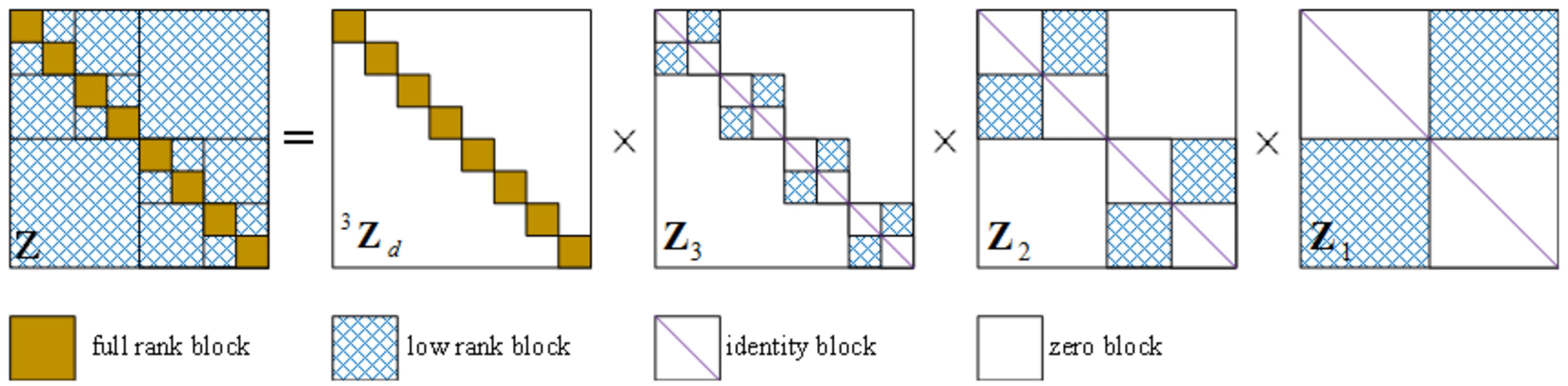
Fig. 3. A division of the initial matrix Z with a three-level binary tree.

Size of both ${}^1\mathbf{Z}_{11}$ and ${}^1\mathbf{Z}_{22}$ are $N\mathrm{/}2$, which means the direct calculation of the inverse is also expensive for large N. So just like what is done for the initial matrix Z, using the one-level SMWA to calculate the inverse of ${}^1\mathbf{Z}_{11}$ and ${}^1\mathbf{Z}_{22}$ until the size of the self-impedance matrix block is considered small enough. That is the multilevel version of the SMWA [12]-[14]. If a q-level binary tree is taken, the initial matrix Z can be represented as the multiplication of a series of matrices

$$\mathbf{Z}{=}^q{\mathbf{Z}}_d{\mathbf{Z}}_q\mathrm{\cdots }{\mathbf{Z}}_3{\mathbf{Z}}_2{\mathbf{Z}}_1.$$

(35)

The pictorial representations of the matrices in the SMWA with a three-level binary tree are shown in Figure 3. Eventually, the linear system (26) can be efficiently calculated as

$${\mathbf{Z}}^{-1}\mathbf{B}={\mathbf{Z}}_1^{-1}{\mathbf{Z}}_2^{-1}{\mathbf{Z}}_3^{-1}\mathrm{\cdots }{\mathbf{Z}}_q^{-1}{}^q\mathbf{Z}_d^{-1}\mathbf{B}.$$

(36)

Fig. 4. The bistatic RCS of a sphere with radius 1.0 m entirely coated by the thin material with $d=0.0125$m, ${\epsilon }_r=4$ and ${\mu }_r=4$.

III NUMERICAL RESULTS

This section is divided into two parts. The first part is to verify the correctness of our code. And then the second part is to illustrate the effectiveness of our work. The example to validate our code is to calculate the bistatic RCS of a PEC sphere of radius 1.0 m, but entirely coated by the material with $d=0.0125$m, ${\epsilon }_r=4$ and ${\mu }_r=4$. The coated sphere is illuminated by an x-polarized incident plane wave from the direction at ${\theta }_i=0{}^{\circ }$, ${\phi }_i=0{}^{\circ }$ with a frequency at 300 MHz, and only the PEC surface of the sphere is discretized into flat triangles with the mean size of $0.1{\lambda }_0$. ${\lambda }_0$ is the wavelength in free space. The results are shown in Figure 4. It can be seen that the RCS calculated by our code matches the solution of the business software FEKO well.

Fig. 5. The bistatic RCS of a simplified missile model with different coating positions.

In the next step, different coating conditions will be discussed. One example is analyzing the bistatic RCS of a simplified missile model with different coating location to demonstrate the efficiency of the proposed method. The tolerance of the ACA algorithm is ${10}^{-4}$. A level-6 binary tree is employed. The model consists of a cylinder, a hemisphere and several cuboids, as shown in Figure 5. The cylinder is 5.0 m high with a radius of 0.25 m, and the radius of the hemisphere is 0.25 m. The cuboid at the middle of a cylinder is 2.6 m long, 0.05 m wide, and 0.3 m high and its long side is parallel to the x-axis. The cuboid at the tail is 1.5 m long, 0.05 m wide, and 0.2 m high. The head of the missile is facing positive z-axis. The missile model is illuminated by an x-polarized incident plane wave from the direction at ${\theta }_i=0{}^{\circ }$, ${\phi }_i=0{}^{\circ }$, with a frequency of 1.0 GHz. The discrete size is $0.1{\lambda }_0$. This model contains 33,648 RWGs. Five positions are selected for the coating and each time only one position is coated. The first position is the head of the missile. The rest of the position is one position every 0.5 m from the head down on the cylinder surface. The relative permittivity, relative permeability, and thickness of coated material are ${\epsilon }_r=2-j1$, ${\mu }_r=2-j1$, and $d=0.0075$m, respectively.

Figure 5 shows the result in position 1 that a good agreement can be found by comparing the proposed method and the conventional method [6], [7]. Table 1 gives the CPU time consumption. The conventional method directly applies the LU decomposition to calculate the solution. The proposed method takes the same amount of time as the conventional method for computing the voltage and impedance matrix, however, the time saved is in the solution. When the analysis of five changes are completed, the total computational time is saved by more than half by the proposed method. Why the time of LU in conventional method looks the same is because the total unknown is the same each time. The conventional method has a maximum memory footprint of 8650 MB for one coating situation while the proposed method has 4970 MB.

Table 1: CPU time for different coating positions

Coating position	Conventional method		Proposed method
	Voltage and	LU	Voltage and	Solve
	impedance		impedance
	generation		generation
PEC	1296 s		836 s
1	164 s	746 s	164 s	54 s
2	283 s	747 s	283 s	100 s
3	280 s	747 s	280 s	100 s
4	280 s	746 s	280 s	101 s
5	281 s	752 s	281 s	100 s
Total	6325 s		2579 s

IV CONCLUSION

In this paper, an efficient method for analyzing the scattering of a PEC object with partial different thin coatings is presented. The proposed method only needs to calculate the inverse of PEC matrix once, which can be reused to efficiently acquire the outcome of local thin coating at different locations or with different electromagnetic parameters. In the proposed method, the employment of the SMWA speeds up the calculation of the inverse of the PEC matrix, which further accelerates the solution. For analyzing a PEC object with partial and thin coatings, the proposed method has a remarkable enhancement in computing time and memory requirement compared with the conventional method [6], [7].

ACKNOWLEDGMENT

This work was supported by the Fundamental Research Funds for the Central Universities (NS2020028), the National Nature Science Foundation of China (61771238), the Joint Open Project of KLME & CIC-FEMD, NUIST (KLME201910), the Foundation of State Key Laboratory of Millimeter Waves, Southeast University, China, (K202035), and the Project of Key Laboratory of Radar Imaging and Microwave Photonics (Nanjing University of Aeronautics and Astronautics), Ministry of Education (RIMP2020006), the Open Fund of Graduate Innovation Base for Nanjing University of Aeronautics and Astronautics (KFJJ20200418). Thanks to Altair for providing software and technical support.

References

[1] W. C. Gibson, The Method of Moments in Electromagnetics. Boca Raton, FL, USA: CRC Press, Nov. 2007.

[2] O. Ergul and L. Gurel, The Multilevel Fast Multipole Algorithm (MLFMA) for Solving Large-Scale Computational Electromagnetics Problems. John Wiley & Sons, Apr. 2014.

[3] C. C. Lu and W. C. Chew, “A coupled surface-volume integral equation approach for the calculation of electromagnetic scattering from composite metallic and material targets,” IEEE Trans. Antennas Propag., vol. 48, no. 12, pp. 1866-1868, Dec. 2000.

[4] I. Chiang and W. C. Chew, “Thin dielectric sheet simulation by surface integral equation using modified RWG and pulse bases,” IEEE Trans. Antennas Propag., vol. 54, no. 7, pp. 1927-1934, Jul. 2006.

[5] I. Chiang and W. C. Chew, “A coupled PEC-TDS surface integral equation approach for electromagnetic scattering and radiation from composite metallic and thin dielectric objects,” IEEE Trans. Antennas Propag., vol. 54, no. 11, pp. 3511-3516, Nov. 2006.

[6] S. Tao, Z. Fan, W. Liu, and R. Chen, “Electromagnetic scattering analysis of a conductor coated by multilayer thin materials,” IEEE Antennas Wirel. Propag. Lett., vol. 12, pp. 1033-1036, Aug. 2013.

[7] S. Tao, D. Ding, and R. Chen, “Electromagnetic scattering analysis of a conductor coated by thin bi-isotropy media,” Microw. Opt. Technol. Lett., vol. 55, no. 10, pp. 2354-2358, Oct. 2013.

[8] W. Hager, “Updating the inverse of a matrix,” SIAM Rev., vol. 31, no. 2, pp. 221-239, Jun. 1989.

[9] E. Yip and B. Tomas, “Obtaining scattering solution for perturbed geometries and materials from moment method solutions,” Applied Computational Electromagnetics Society (ACES) Journal, vol. 3, no. 2, pp. 95-118, Jul. 1988.

[10] A. Boag, A. Boag, E. Michielssen, and R. Mittra. “Design of electrically loaded wire antennas using genetic algorithms,” IEEE Trans. Antennas Propag., vol. 44, no. 5, pp. 687-695, May 1996.

[11] X. Chen, X. Liu, Z. Li, and C. Gu, “Efficient calculation of interior scattering from cavities with partial IBC wall,” Electronics Letters, vol. 56, no. 17, pp. 871-873, Aug. 2020.

[12] X. Chen, C. Gu, Z. Li, and Z. Niu, “Accelerated direct solution of electromagnetic scattering via characteristic basis function method with Sherman-Morrison-Woodbury formula-based algorithm,” IEEE Trans. Antennas Propag., vol. 64, no. 10, pp. 4482-4486, Oct. 2016.

[13] W. Y. Kong, J. Bremer, and V. Rokhlin, “An adaptive fast direct solver for boundary integral equations in two dimensions,” Appl. Comput. Harmon. Anal., vol. 31, no. 3, pp. 346-369, Jan. 2011.

[14] S. Ambikasaran and E. Darve, “An O(NlogN) fast direct solver for partial hierarchically semi-separable matrices,” J. Sci. Comput., vol. 57, no. 3, pp. 477-501, Apr. 2013.

[15] M. Bebendorf, “Approximation of boundary element matrices,” Numer. Math., vol. 86, no. 4, pp. 565-589, Jun. 2000.

[16] K. Zhao, M. Vouvakis, and J.-F. Lee, “The adaptive cross approximation algorithm for accelerated method of moments computations of EMC problems,” IEEE Trans. Electromagn. Compat., vol. 47, no. 4, pp. 763-773, Nov. 2005.

[17] S. Rao, D. Wilton, and A. Glisson, “Electromagnetic scattering by surfaces of arbitrary shape,” IEEE Trans. Antennas Propag., vol. AP-30, no. 3, pp. 409-418, May 1982.

ACES JOURNAL, Vol. 36, No. 10, 1274–1280.
doi: 10.13052/2021.ACES.J.361002
© 2021 River Publishers

Abstract

I INTRODUCTION

II FORMULATION

A Conventional method for PEC with thin coating

B Efficient method for PEC with partial and thin coating

III NUMERICAL RESULTS

IV CONCLUSION

ACKNOWLEDGMENT

References