Advanced Numerical and Experimental Analysis of Ultra-Miniature Surface Resonators
Yakir Ishay, Yaron Artzi, Nir Dayan, David Cristea, and Aharon Blank
Schulich Faculty of Chemistry
Technion - Israel Institute of Technology, Haifa, 3200003, Israel
yakir387@gmail.com, yaron160@gmail.com, nirdayan11@gmail.com, cristea.david@gmail.com, ab359@technion.ac.il
Submitted On: October 14, 2021; Accepted On: August 11, 2022
Abstract
Many scientific and technological applications make use of strong microwave fields. These are often realized in conjunction with microwave resonators that have small geometric features in which such fields are generated. For example, in magnetic resonance, large microwave and RF magnetic fields make it possible to achieve fast control over the measured electron or nuclear spins in the sample and to detect them with high sensitivity. The numerical analysis of resonators with small geometric features can pose a significant challenge. This paper describes a general method of analysis and characterization of surface microresonators in the context of electron spin resonance (ESR) spectroscopy and spin-based quantum technology. Our analysis is based on the Electric Field Integral Equation (EFIE) and the Poggio-Miller-Chang-Harrington-Wu-Tsai (PMCHWT) formulation. In particular, we focus on a class of resonator configurations that possesses extremely small subwavelength features, which normally would require an ultra-fine mesh. We present several efficient techniques to numerically model, solve, and analyze these types of configurations for both normal and superconducting structures. The validation of these techniques is established both numerically and experimentally by the S parameters as well as the provision of direct mapping of the resonator’s microwave magnetic field component using a unique electron spin resonance micro-imaging method.
Index Terms: electric field integral equation, electron spin resonance, surface resonators.
I. INTRODUCTION
Surface microresonators belong to a subclass of planar printed resonators [1]. They constitute a key component in many scientific and technological applications ranging from filters [2] and oscillators [3] for analog and digital communications to building blocks for metamaterials [4] and including quantum technology [1, 6]. Essentially, this is a result of the richness of resonator topologies, which can be generated and rendered optimal for various uses. Indeed, recent advances in fabrication techniques [7] and lower manufacturing costs allow designing such surface resonator configurations to obtain the desired microwave (MW) field distribution in a certain bandwidth (BW).
One of the emerging fields of application of surface resonators is magnetic resonance and specifically electron spin resonance (ESR) [8]. This method makes use of such resonators to focus the microwave magnetic field component on a small region in space [9], thereby increasing the effectiveness, and especially the sensitivity, of ESR [10, 11]. The capability to generate specific MW magnetic field patterns can be useful in a variety of ESR applications such as the detection and imaging of defects on the surface and subsurface of semiconductors [12], measurements of paramagnetic monolayers [13], and the inspection of small biological systems [14]. Many types of ESR surface resonators are often comprised of a mixed structure of metallic and dielectric parts and characterized by areas with small geometric features that can range from 0.01 to even 10, where is the operating wavelength. In terms of full Electromagnetic (EM) simulation, this results in an ultra-fine mesh in and around these areas. Therefore, achieving an accurate numerical solution presents a difficulty that in many applications, and especially in ESR, may be critical. Primarily, this is because the system’s ultimate performance is determined by the resonator’s properties such as its filling factor [15]:
where H is the component of the MW magnetic field that is tangential to B, the direction of the static field, and |H| is the modulo of the MW magnetic field. This means that finding requires an accurate solution of the resonant MW fields all over the resonator, both near and far from its core.
Another difficulty originates in the inclusion of a long (several wavelengths) excitation device (typically a microstrip line), which further amplifies the need to address the challenge of having objects with dimensions spanning many orders of magnitude with respect to . Our experience has shown that for these types of EM problems, leading commercial EM solvers such as CST or HFSS, which are based on the Finite Difference Time Domain (FDTD) [16], or Finite Element Method (FEM) [17], frequently fail to achieve a numerical solution with the desired degree of accuracy within a reasonable time frame. Essentially, this is because such a solution requires a very fine mesh across most of the volume defined by the boundary box. Numerical solvers based on Method of Moments (MoM) [18] and Surface Integral Equation (SIE) [19] methods can solve this obstacle given that once the surface currents are known, it is possible to have accurate data throughout the entire space. Yet, naively employing MoM solvers is not sufficient, in particular for configurations of surfaceresonators with an overall size of 0.1 that have 10 features whose numerical solution involves solving a matrix system with an extremely high condition number (10–10).
Here, we present a numerical MoM-SIE solver based on the Electric Field Integral Equation (EFIE) [20] and the Poggio-Miller-Chang-Harrington-Wu-Tsai (PMCHWT) [21, 22] formulation for general composite structures that have been optimized for EM problems involving the complex geometries common in the field of ESR surface resonators. This paper aims to present our advanced techniques for obtaining an accurate and efficient numerical solution to these challenging types of EM problems while providing experimental validation of the theoretical results. The increased efficiency with respect to calculation time and memory usage is revealed when comparing our algorithm to the industry standard CST frequency domain and integral equation solvers. This efficiency is attributed to three main features of this work: (i) the achievement of reasonable condition numbers by applying proper model discretization, even for very fine physical features; (ii) the application of unique procedures for matrix system preconditioning; and (iii) the implementation of Impedance Boundary Conditions (IBC) to represent thin conductors as a surface impedance to exclude ultra-small elements that significantly increase the impedance matrix condition number and to account for lossy realistic structures.
II. EFIE-PMCHWT SURFACE INTEGRAL EQUATIONS
A. Formulation
The EFIE-PMCHWT formulation applies the EFIE to open/closed metallic surfaces and the PMCHWT to dielectric domains [23]. Closed metallic surfaces can also be treated with the Combined Field Integral Equation (CFIE) [24] to remove interior resonances. However, thin conductors are required to be modeled as open surfaces, either to make use of Impedance Boundary Conditions (IBC) [25] or because they practically cannot be modeled as closed surfaces, as explained in Section 3.2. Here, the EFIE-PMCHWT equations are reviewed with respect to the following EM scattering problem, illustrated in Fig. 1. Consider a time-harmonic regime with a time factor e and a primary or incident field (E, H) illuminating domains D, D immersed in an unbounded background medium D whose impedance is . Here, D represents a thin conductor modeled as an open surface S with surface impedance Z. S is assumed to have a radius of curvature that is large compared to the operating wavelength . D denotes a dielectric domain enclosed by a surface S with material properties and . Let E and H be the secondary microwave fields generated by J and M representing electric and magnetic surface currents, respectively. We define integral operators T and K associated with region i [0,1], acting on vector field F across a surface S, by [20, 24]
| (1) | ||
| (2) |
Here, the surface normal of is the Green’s function of an infinite homogeneous medium with wavenumber given by:
| (3) |
and I represents the identity operator.
For conductors with , the boundary condition on can be approximated as [25]:
| (4) |
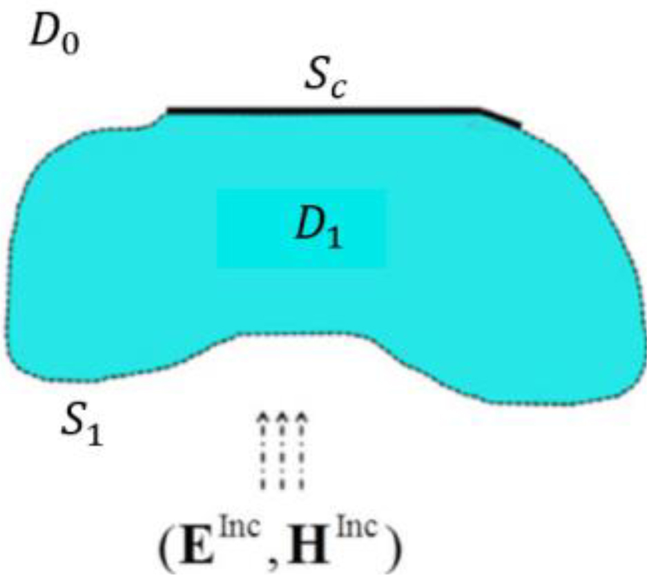
Figure 1: Scattering by composite conductor and dielectric structures. The solid black line corresponds to an open surface S modeling a thin conductor associated with a domain D. The dashed line corresponds to a surface S enclosing a dielectric domain D.
and on the surface S the boundary conditions read [21]:
| (5) |
| (6) |
with being the impedance of region i. Equation (4) represents the EFIE and (5) and (6) represent the PMCHWT.
B. Discretization
The numerical solution is obtained by transforming the EFIE-PMCHWT equations (4), (5), and (6) into a matrix system. First, J and M are approximated in terms of vector basis functions:
| (7) |
where f is the Rao-Wilton-Glisson (RWG) basis function [20] assigned to the edge e defined as (Fig. 2).
| (8) |
Here, is the area of the triangular patch is the length of the common edge , and is the vertex of . An RWG function domain is displayed in Fig. 2. The a and b parameters are associated with N unknown electric and N magnetic current amplitudes, respectively. The values of N and N are determined by the number of edges associated with each surface so that N corresponds to both conductor and dielectric surfaces S S, whereas N applies only to S = S \ S. The latter condition applies only for conductors with |Z|, where the magnetic edges lying in S are removed (note that for their correct removal, the meshes applied to opposite sides of the interface must be identical). To discretize the EFIE-PMCHWT equations, the Galerkin method is applied so that (4), (5), and (6) are tested using f, e S, f, e S, and f, e S, respectively. This procedure results in the following matrix equation:
| (9) | ||
| (10) | ||
| (11) |
Here we define:
| (12) | ||
| (13) | ||
| (14) | ||
| (15) | ||
| (16) |
Hence, the impedance matrix is of the form:
| (17) |
where the elements of the block matrices are:
| (18) | |
| (19) | |
| (20) | |
| (21) | |
| (22) | |
| (23) |
The evaluation of the double integrals (12) to (16) is performed using the singularity subtraction technique with closed-form integral representations [26].

Figure 2: An RWG function f composed of a pair of triangular patches and common to the n edge e.
III. SIMULATION OF ESR RESONATOR CONFIGURATIONS
A. Model
ESR surface resonators typically operate in the range of 1–100 GHz where their size is, in most cases, much smaller than the resonant wavelength. Figure 3 shows a typical layout of the “ParPar” (“butterfly” in Hebrew) surface resonators we have recently developed [27]. It consists of a thin (50–500 nm) butterfly-shaped conductor (either normal or superconductor) printed on a thick (100–500 m) dielectric substrate whose width/length is typically 1.2 – 1.6 mm The bridge (at the center of Fig. 3 (a)) is chosen so that it maximizes the magnetic field in a particular region of thin ( 200 m) samples that cover the resonator plane(i.e., the substrate’s upper plane). The resonators are inductively coupled by a microstrip line placed 10 – 300 m below the substrate’s bottom plane, where critical (optimal) coupling [28] can be achieved by moving the resonator in the x-y plane (Fig. 3 (b)). The microwave configuration composed of a surface resonator and a microstrip transmission line can be represented by the equivalent circuit shown in Fig. 4.
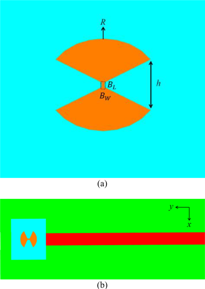
Figure 3: ESR microwave configuration. (a) General layout of the ParPar surface resonator. The dashed rectangular line indicates the bridge whose length and width are B and B, respectively. The arcs’ radii R and h denote the complementary physical characteristics of the ParPar resonator. (b) Excitation of ParPar by a microstrip line.
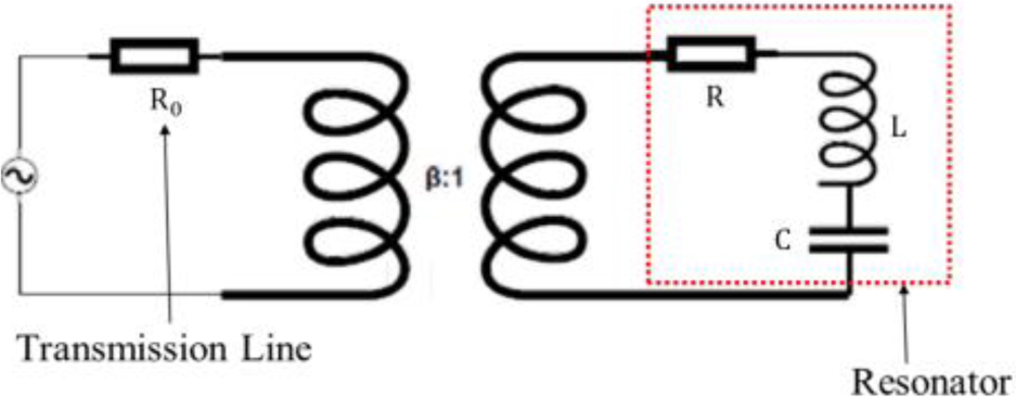
Figure 4: Equivalent circuit for ESR microwave configuration. The microstrip line and surface resonator are represented by the elements R and R, L, and C, respectively. denotes the inductive coupling coefficient.
B. Boundary conditions
Common ESR surface resonators consist of extremely thin conductors (including those associated with the microstrip) whose thickness can be smaller than the penetration depth for normal conductors (e.g., copper, silver, etc.) and the London penetration depth [29] for superconductors1. As a result, the use of Impedance Boundary Conditions (IBC) is critical because modeling the conductors as closed surfaces might result in ill-conditioned matrix systems, as explained in detail in the following subsection. The implementation of IBC is performed using the single sheet model [30], in which the conductor is modeled as a single sheet with the appropriate surface impedance Z. The value of Z depends on the type of conductor (normal or superconductor) used. In the case of normal conductors, the surface impedance is given by [30]:
| (24) |
where is the medium impedance, is the complex conductivity, and = (1+j)/.
For superconductors, the surface impedance is [30]:
| (25) |
The single sheet model can also be applied to either planar or non-planar surfaces whose radii are much greater than the operating wavelength.
Note that regardless of the type of conductor used, the underlying assumption of the boundary impedance model is that the corresponding penetration depth is not much greater than the conductor’s thickness [30]. In this paper, we focus on structures fabricated out of planar normal conductors, while our latest paper [31] deals with resonators made of a superconducting material.
C. Impedance matrix preconditioning and inversion
As mentioned in the previous subsection, the use of IBC alleviates the need for solving ultra-small elements (compared to the operating wavelength) resulting from the inclusion of thin finite conductors. Mathematically, the presence of small elements gives rise to an impedance matrix whose condition number grows as (k) [32]. Here is the weighted average edge length of the mesh so that smaller edges are given more weight. The increase in the condition number results mainly from the EFIE matrix system becoming severely ill-conditioned with increasing mesh density and decreasing element size. In cases where direct solvers cannot be applied (e.g., for large matrix systems), this eventually leads to slowly- or non-converging iterative solvers, namely a dense discretization breakdown [33]. In fact, the mesh applied to a specific model is of importance, and this is especially true for MoM-based integral equations solvers [34–36]. However, numerically solving a microwave configuration composed of an electrically large microstrip line and a small surface resonator possessing fine and localized geometric features still requires solving a large impedance matrix whose condition number is considerably high (e.g., 10–10 when solving typical ParPar layouts, as described above). Furthermore, the resulting MW fields are required to be very accurate within the sample volume and at least 1 m spatial resolution is necessary for resolving ultra-small samples (i.e., with volume 1 nL). Therefore, the impedance matrix must be preconditioned properly to improve its condition number and enable an accurate solution to the problem.
Theoretically, preconditioning can be based either on simple algebraic techniques, such as incomplete LU (ILU) factorization [37, 38] or approximate inverse preconditioners [39] or on a more physical class of preconditioners, such as the Calderon Multiplicative Preconditioner (CMP) [40]. On the one hand, under quasi-uniform discretization, Calderon identity-based preconditioners might result in a condition number whose upper bound can be independent of [41], while algebraic preconditioners still exhibit a growing condition number as decreases. On the other hand, CMP might not be applicable to these types of problems for the following reasons: first, improving the condition number in the presence of a non-uniform mesh is not guaranteed, given that the CMP-EFIE method still suffers from an inaccuracy problem at low frequencies associated with quasi-static regions [42, 43], and imposing a uniform mesh is not practical, especially in complex ESR resonators geometries. Second, employing CMP for open surfaces is less effective because the condition number might grow similarly to the EFIE matrix system [44]. Third, for a matrix system that can be preconditioned algebraically, applying CMP can be a time-consuming procedure due to an excess in matrix-matrix and matrix-vector products. Fourth, CMP might not be trivially extended for EFIE-PMCHWT formulations, whereas an extra challenge is added by the inclusion of IBC. The latter also applies to other formulations, such as multiple-traces PMCHWT [45], that can lead to a well-conditioned impedance matrix in configurations comprising perfectly conducting objects.
As shown in Section IV.C below, a matrix preconditioned via an incomplete LU factorization can significantly improve its condition number. In particular, compared to the left ILU preconditioner, which multiplies the impedance matrix on the left, the right ILU preconditioner is much more efficient and provides exceptional iterative solver convergence speed: up to 30 GMRES iterations to achieve relative residuals min (10, condition number) with respect to the unpreconditioned matrix system. Calculating the residual in this manner excludes either delayed or premature convergence associated with left preconditioners [46]. Typically, for condition numbers 10, the left ILU becomes less practical due to slow convergence and an inaccurate numerical solution compared to the right ILU. Moreover, the standard diagonal preconditioner (DP) cannot resolve condition numbers 10 and results in non-convergence. Mathematically, solving configurations near resonance requires a substantial decrease in the matrix’s high condition number, which cannot be achieved by decreasing the dominance of its diagonal alone. However, the DP can lower the condition number by 2 – 3 orders of magnitude; therefore, it can be applied prior to the left ILU preconditioner to enhance convergence.
As for the particular iterative solver to be used, there are several methods to choose from, including the generalized minimum residual (GMRES) method proposed by Saad and Schultz [47], the biconjugate gradient (BiCG) developed by Fletcher [48], the conjugate gradient squared (CGS) method proposed by Sonneveld [49], the transpose-free quasiminimal residual method (TFQMR) by Freund and Nachtigal [50], and van der Vorst’s gradient stabilized (BiCGSTAB) [51] method. While they are applicable to our problems, GMRES with right ILU preconditioning has provided the fastest convergence. Accordingly, in this work, we employed GMRES with residue tolerance of min(10, condition number) following ILU factorization performed with pivoting (ILUP [47]) and drop tolerance of 10.
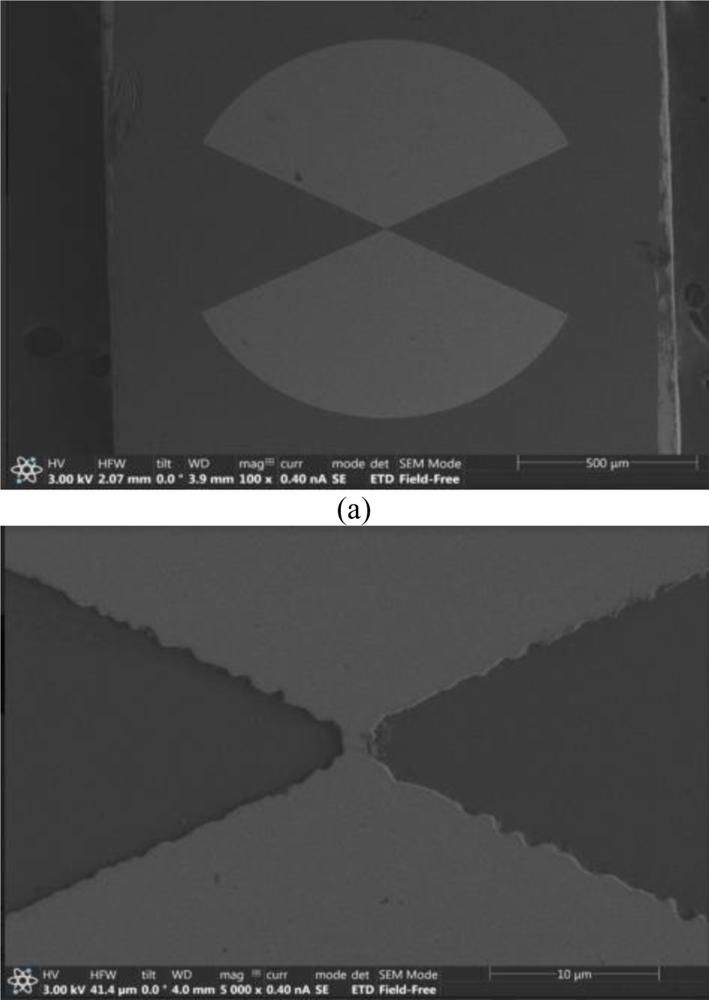
Figure 5: SEM photos of ParPar2 surface resonators. (a) Low magnification. (b) High magnification.
IV. NUMERICAL & EXPERIMENTAL RESULTS
A. ParPar topology
This section presents numerical and experimental results that demonstrate the time efficiency and the accuracy of our method to resolve complex ESR microwave resonator configurations. In particular, we show accurate near-field solutions that were validated via a sensitive and unique ESR microimaging setup. Three types of ParPar surface resonators were tested: ParPar50, ParPar20, and ParPar2, whose bridge sizes (B, B – see Fig. 3 (a)) are (25 m, 50 m), (10 m, 20 m), and (1 m, 2 m), respectively. Each of these resonators consisted of a 0.5 m-thin copper metallization printed on LaAlO or silicon dielectric substrates (1.6 mm 1.6 mm 0.2 mm) with permittivity of 24 and 11.5, respectively. The arcs’ radii R (Fig. 3 (a)) were 380 m for the LaAlO substrate, and 560 m for the silicon substrate. Figures 5 (a) and 5 (b) show the scanning electron microscope (SEM) photos of the ParPar2 resonator for illustration purposes. Coupling to the resonators was achieved via a 0.46 mm-wide microstrip line (RO4003 LoPro Series, Rogers Corp., thickness of 0.22 mm) whose end was placed 10 m, 12 m, and 190 m below the substrate’s bottom plane for ParPar50, ParPar20, and ParPar2, respectively. Note that an inductive coupling to ParPar2 is much more challenging, considering the magnetic flux generated by the millimeter-scale microstrip line. The comparison between measured and calculated reflection coefficients S is presented in Figs. 6 and 7; in all cases (Figs. 6 (a) to 6 (c) and 7 (a) to 7 (c)), the resulting maximal relative error between the measured and calculated S is 2% in the resonance and 5% in the 3 dB BW. This fine agreement is definitely not trivial, in particular for the ParPar2 resonator whose structure was discretized with an average element /50 in size (minimum edge length of 310), resulting in a MoM matrix condition number of 10. The calculated resonant magnetic field distributions for ParPar50, ParPar20, and ParPar2 geometries are presented in Figs. 8 (a) to 8 (c), respectively. Evidently, in all cases, the magnetic field is mostly localized in and around the bridge. The pattern of this mode can be verified via 2D ESR microimaging [52], considered to be a very sensitive method to reveal the intensity of the actual microwave magnetic field. Additional details about the ESR imaging procedure used in this work are provided in the Appendix. For example, results of the imaging experiments carried out with ParPar50 and ParPar2 (Fig. 9) showed that the desired mode is indeed excited in both cases.
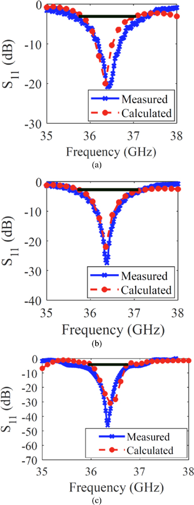
Figure 6: Measured and calculated reflection coefficient S for LaAlO resonators. (a) ParPar50, (b) ParPar20, and (c) ParPar2.
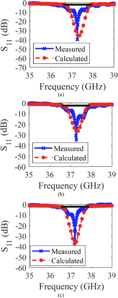
Figure 7: Measured and calculated reflection coefficient S for silicon resonators. (a) ParPar50, (b) ParPar20, and (c) ParPar2.
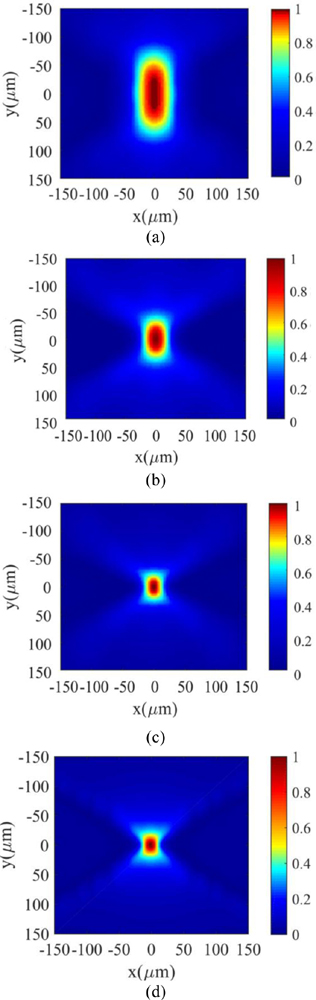
Figure 8: Calculated normalized magnitude of resonant magnetic field distributions 16 m, 8 m, and 4 m above the substrate’s upper plane for (a) silicon-ParPar50, (b) LaAlO-ParPar20, and (c) LaAlO-ParPar2, respectively. (d) The corresponding CST results for LaAlO-ParPar2.
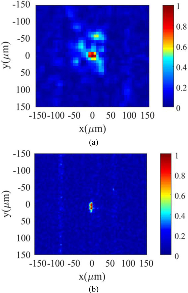
Figure 9: Results of ESR microimaging carried out with (a) ParPar50 using a silicon substrate and (b) ParPar2 using LaAlO. Both resonators were covered completely by a sample consisting of paramagnetic microcrystals, which resulted in a non-uniform (grainy) mode image. A detailed description of the experiments can be found in the Appendix.
B. Impedance matrix preconditioning
In this section, we demonstrate our method’s capability to solve the high condition number matrices resulting from the discretization of ParPar2 and ParPar20 surface resonators (LaAlO substrate). On both structures, the simulations were repeated for 11 non-uniform discretizations with an average edge length that varied from 0.02 to 0.05 , corresponding to 4016 RWG functions for the largest and 16248 for the smallest. Here, is the resonant wavelength at 36.3 GHz For all discretizations, the minimum edge lengths were kept the same—310 and 310 for ParPar2 and ParPar20, respectively. Figure 10 (a) presents the resulting condition numbers of the EFIE-PMCHWT matrices for simulated ParPar2 and ParPar20. Regarding Fig. 10 (a), the minimum condition number (10) of the ParPar2 impedance matrix is 2 orders of magnitude larger than the maximum condition number of the ParPar20 matrix. These results clearly suggest that discretizations having a lower -to- ratio are significantly more susceptible to higher condition numbers than more uniform discretizations with smaller values. In practical terms, this means that extra mesh refinements of subwavelength regions, which correspond to an excessive presence of smaller elements, can greatly impair the quality of the numerical solution. Figure 10 (b) presents the performance of the diagonal preconditioner (DP) with left and right ILU ILU applied to resolve the high condition numbers of the impedance matrix for the aforementioned discretizations of ParPar2. Applying the right ILU allows for the convergence of GMRES (relative residual condition number) on every discretization, while the left ILU preconditioner becomes less effective for dense discretizations so that the GMRES residual gradually increases and surpasses 10. Thus, while memory usage for the left and right ILU were quite similar, the right ILU typically required 15 iterations to converge, for all examined discretizations, whereas the left ILU resulted in 30 iterations and non-convergence (a stagnation of the GMRES) for condition numbers 10, and 10, respectively. Note that using DP alone could not resolve these high condition numbers, even for the coarsest discretization. Namely, the iterative solver did not converge when attempting to solve the diagonally preconditioned impedance matrix. In practice, we found the tolerance of 10 to be unachievable by GMRES, which stagnated after 300 iterations
Lastly, to illustrate the importance of the right ILU preconditioner, we attempted to solve the ParPar2 structure for extremely fine discretization—32450 RWG functions at a resonance of 36.3 GHz While the GMRES stagnated following 800 iterations using the left ILU, for the right ILU-preconditioned impedance matrix we achieved GMRES convergence following 101 iterations. Therefore, we conclude that the left ILU preconditioner can be ineffective to solve complex structures near resonance, in particular for very fine discretizations and large matrices.
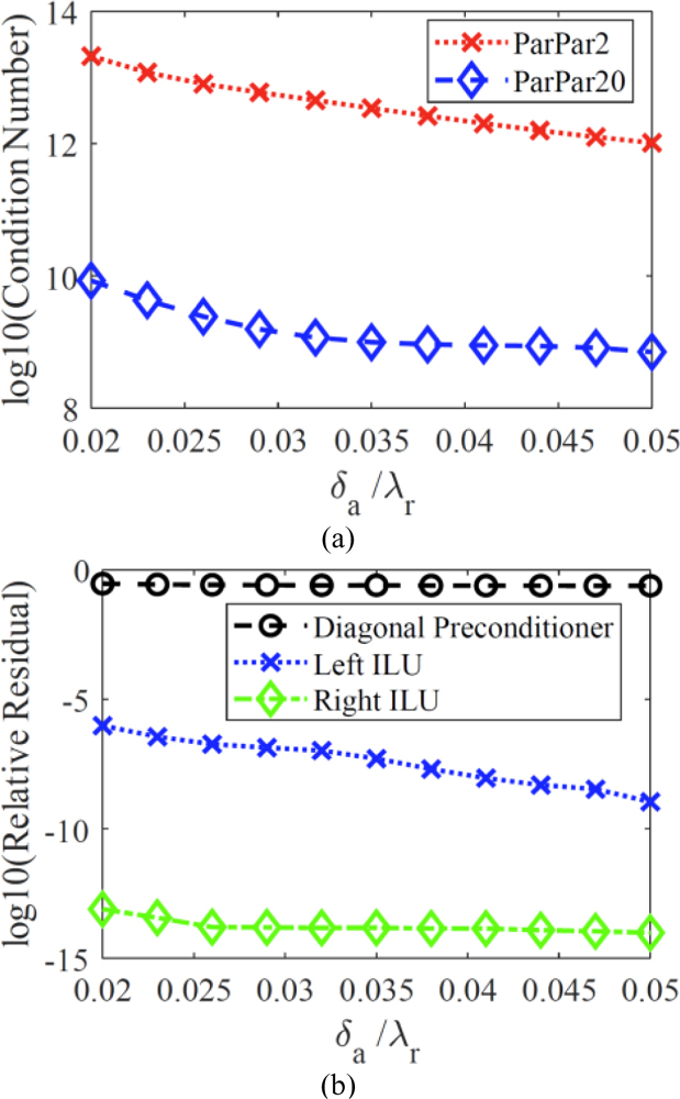
Figure 10: Performance of the DP with left and right ILU to precondition the EFIE-PMCHWT impedance matrix of ParPar20 and ParPar2. (a) Condition number of ParPar20 and ParPar2 impedance matrices. (b) GMRES residual following 30 iterations.
C. Comparison with CST
In the last section, our MoM-based solver is compared with the CST Frequency Domain Solver (Fsolver) via simulation of the configuration composed of the LaAlO-ParPar2 resonator and a microstrip line described in previous sections. Both solvers were compared regarding simulation time per frequency point (STPFP) and the number of unknowns (NoU) resolved for near-field and S convergence (i.e., 0.2% norm variation), where near-field convergence was tested using 10 grid points within a 1.6 mm 1.6 mm 100 m sample volume situated above the resonator’s surface. Figure 8 (d) shows the corresponding CST results depicting the resonant magnetic field distribution (respective to Fig. 8 (c)). All simulations were carried out on a 3.2 GHz Intel Xeon 1660 processor. The results are summarized in Table 1.
It is evident from Table 1 that while our MoM solver required the same NoU for both S and near-field convergence, the CST Fsolver required almost double NoU to converge in the near-field region. Moreover, for CST, an additional manual mesh refinement was required at the center of the resonator, as it was not refined properly during the adaptive mesh refinement process. 650774757Note that being an FEM-based method,the CST
Fsolver divided the geometric model into a large number of tetrahedra within a predefined bounding box—a property that results in a very large matrix system to solve. In terms of simulation time, both solvers were comparable regarding STPFP (210–270 s) to achieve S convergence. However, the STPFP of the CST Fsolver for nearfield convergence was 430 s, due to the need for a much finer mesh in the sample region. Furthermore, the total simulation time per frequency point plus the duration required for the adaptive mesh refinement process for the Fsolver was typically 1 hour due to the time-consuming adaptive mesh refinement process. Contrastingly, in the case of EFIE-PMCHWT, the total simulation time and STPFP were equivalent. We also note that the MoM solver greatly outperformed the CST Fsolver when applying the right ILU as a preconditioner, whereas a left ILU-preconditioned impedance matrix resulted in very slow convergence of the iterative solver—the STPFP was 4 times larger than the corresponding right ILU preconditioner. The total simulation times calculated for 21 frequency steps in a range of 34–39 GHz were approximately 210 minutes (including the adaptive mesh process) in CST and 37 minutes in the EFIE-PMCHWT solver employing the right ILU as a preconditioner. The relatively short simulation time of the EFIE-PMCHWT solver is due to the computation of the singularity extraction, which was executed once for any given frequency band [26].
Lastly, we also attempted to use CST with the Integral Equation Solver (Isolver) to solve the ParPar2. Unfortunately, the results were not correct for the near-field region. Note that to make a fair comparison, the Isolver results were obtained with approximately the same NoU as our MOM solver. However, as explained in Section 3.3, performing a simulation with a finer mesh would probably not provide better results because it would lead to higher condition numbers, which were already very high owing to the complex geometry and near-resonance state.
Table 1: Comparative typical simulation times for the ParPar2 configuration. The STPFP does not include the initial calculation required for mesh refinement
| EM Solver | S11 convergence | Near-field convergence | ||
|---|---|---|---|---|
| NoU | STPFP [s] | NoU | STPFP [s] | |
| CST Fsolver | 270,000 | 270 | 600,000 | 431 |
| EFIE-PMCHWT | 4828 | 210 | 4828 | 210 |
V. CONCLUSION
In this work, we developed an efficient methodology using a modified EFIE-PMCHWT formulation with impedance boundary conditions to solve surface MW resonators with dimensions and features that span several orders of magnitude with respect to the operating wavelength. The new methodology was used to solve three complex, realistic resonator configurations. The complexity of these configurations arises from a combination of electrically large structures, such as microstrip lines, and small surface resonators that have subwavelength localized geometric features. These types of configurations require dense and non-uniform discretizations, resulting in an impedance matrix whose condition number is in the range of 10–10. On the one hand, we showed that applying right incomplete LU (ILU) preconditioners can improve dramatically the condition number and thus allow for a fast iterative solver convergence. On the other hand, applying left ILU preconditioners resulted in very slow GMRES convergence, suggesting that left ILU preconditioning is considerably less effective than right ILU for this type of problem. We also showed that the standard diagonal preconditioner (DP) might be impractical for these types of resonator configurations, leading to a non-converging iterative solver. We validated our solution via network analyzer measurements and ESR microimaging experiments. Finally, we showed that for the geometries we tested, the preconditioned EFIE-PMCHWT impedance matrix outperformed the CST frequency domain solver (Fsolver) in terms of simulation time because of the ultra-fine mesh required to achieve near-field convergence in the latter. Moreover, the CST integral equation solver could not provide accurate results in the near field for the configurations we tested.
ACKNOWLEDGMENT
This work was partially supported by Grant #1357/21 from the Israel Science Foundation (ISF), Grant No. AZ 98010 from Forschungskooperation Niedersachsen-Israel, and by a grant from the Technion-Waterloo joint program. This project was also supported by the generosity of Eric and Wendy Schmidt by recommendation of the Schmidt Futures program. A. B. acknowledges the Russell Berrie Nanotechnology Institute (RBNI) at the Technion for supporting the clean room activities. The resonator was fabricated at Technion’s Micro-Nano Fabrication & Printing Unit (MNF&PU). The numerical data of the calculations are available from the authors upon reasonable request.
REFERENCES
[1] T. Ōkoshi, Planar Circuits for Microwaves and Lightwaves, Springer-Verlag, Berlin, New York, 1985.
[2] J.-S. Hong, Microstrip Filters for RF/microwave Applications, 2nd ed., Wiley, Hoboken, NJ, 2011.
[3] L. Young-Taek, L. Jong-Sik, K. Chul-Soo, A. Dal, and N. Sangwook, “A compact-size microstrip spiral resonator and its application to microwave oscillator,” IEEE Microwave and Wireless Components Letters, vol. 12, pp. 375-377, 2002.
[4] J. Garcia-Garcia, J. Bonache, I. Gil, F. Martin, M. C. Velazquez-Ahumada, and J. Martel, “Miniaturized microstrip and CPW filters using coupled metamaterial resonators,” IEEE Transactions on Microwave Theory and Techniques, vol. 54, pp. 2628-2635, 2006.
[5] R. Vrijen, E. Yablonovitch, K. Wang, H. W. Jiang, A. Balandin, V. Roychowdhury, T. Mor, and D. DiVincenzo, “Electron-spin-resonance transistors for quantum computing in silicon-germanium heterostructures,” Phys. Rev. A, vol. 62, pp. 012-306, 2000.
[6] V. Ranjan, S. Probst, B. Albanese, A. Doll, O. Jacquot, E. Flurin, R. Heeres, D. Vion, D. Esteve, J. J. L. Morton, and P. Bertet, “Pulsed electron spin resonance spectroscopy in the Purcell regime,” J. Magn. Reson., vol, 310, pp. 106-662, 2020.
[7] V.-C. Su, C. H. Chu, G. Sun, and D. P. Tsai, “Advances in optical metasurfaces: fabrication and applications [Invited],” Opt Express, vol. 26, pp. 13148-13182, 2018.
[8] J. A. Weil and J. R. Bolton, Electron Paramagnetic Resonance: Elementary Theory and Practical Applications, 2nd ed., Wiley-Interscience, Hoboken, NJ, 2007.
[9] Y. Twig, E. Suhovoy, and A. Blank, “Sensitive surface loop-gap microresonators for electron spin resonance,” Rev. Sci. Instrum., vol. 81, pp. 104-703, 2010.
[10] Y. Artzi, Y. Twig, and A. Blank, “Induction-detection electron spin resonance with spin sensitivity of a few tens of spins,” Appl. Phys. Lett., vol. 106, pp. 84-104, 2015.
[11] S. Probst, A. Bienfait, P. Campagne-Ibarcq, J. J. Pla, B. Albanese, J. F. D. Barbosa, T. Schenkel, D. Vion, D. Esteve, K. Molmer, J. J. L. Morton, R. Heeres, and P. Bertet, “Inductive-detection electron-spin resonance spectroscopy with 65 spins/root Hz sensitivity,” Appl. Phys. Lett., vol. 111, 2017.
[12] K. Lips, P. Kanschat, and W. Fuhs, “Defects and recombination in microcrystalline silicon,” Sol. Energy Mater., vol. 78, pp. 513-541, 2003.
[13] M. Mannini, D. Rovai, L. Sorace, A. Perl, B. J. Ravoo, D. N. Reinhoudt, and A. Caneschi, “Patterned monolayers of nitronyl nitroxide radicals,” Inorg. Chim. Acta, vol. 361, pp. 3525-3528,2008.
[14] P. P. Borbat, A. J. Costa-Filho, K. A. Earle, J. K. Moscicki, and J. H. Freed, “Electron spin resonance in studies of membranes and proteins,” Science, vol. 291, pp. 266-269, 2001.
[15] A. Blank, Y. Twig, and Y. Ishay, “Recent trends in high spin sensitivity magnetic resonance,” J. Magn. Reson., vol. 280, pp. 20-29, 2017.
[16] D. M. Sullivan, Electromagnetic Simulation using the FDTD Method, 2nd ed., IEEE Press, John Wiley & Sons, Inc., Hoboken, New Jersey, 2013.
[17] G. Meunier, The Finite Element Method for Electromagnetic Modeling, ISTE, Wiley, London, Hoboken, NJ, 2008.
[18] R. F. Harrington, “The method of moments in electromagnetics,” Journal of Electromagnetic Waves and Applications, vol. 1, pp. 181-200, 1987.
[19] A. W. Glisson, D. Kajfez, and J. James, “Evaluation of modes in dielectric resonators using a surface integral equation formulation,” IEEE Transactions on Microwave Theory and Techniques, vol. 31, pp. 1023-1029, 1983.
[20] S. Rao, D. Wilton, and A. Glisson, “Electromagnetic scattering by surfaces of arbitrary shape,” IEEE Transactions on Antennas and Propagation, vol. 30, pp. 409-418, 1982.
[21] V. Jandhyala, B. Shanker, E. Michielssen, and W. C. Chew, “Fast algorithm for the analysis of scattering by dielectric rough surfaces,” Journal of the Optical Society of America A, vol. 15, pp. 1877-1885, 1998.
[22] A. J. Poggio and E. K. Miller, “Chapter 4 - Integral equation solutions of three-dimensional scattering problems,” in R. Mittra (Ed.), Computer Techniques for Electromagnetics, Pergamon, pp. 159-264, 1973.
[23] P. Yla-Oijala, M. Taskinen, and J. Sarvas, “Surface integral equation method for general composite metallic and dielectric structures with junctions,” Progress in Electromagnetics Research, vol. 52, pp. 81-108, 2005.
[24] J. R. Mautz and R. F. Harrington, “H-Field, E-Field, and combined field solutions for bodies of revolution,” in, Defence technical information center, 1977.
[25] A. W. Glisson, “Electromagnetic scattering by arbitrarily shaped surfaces with impedance boundary conditions,” Radio Science, vol. 27, pp. 935-943, 1992.
[26] R. D. Graglia, “On the numerical integration of the linear shape functions times the 3-D Green’s function or its gradient on a plane triangle,” IEEE Transactions on Antennas and Propagation, vol. 41, pp. 1448-1455, 1993.
[27] N. Dayan, Y. Ishay, Y. Artzi, D. Cristea, E. Reijerse, P. Kuppusamy, and A. Blank, “Advanced surface resonators for electron spin resonance of single microcrystals,” Rev. Sci. Instrum., vol. 89, pp. 124-707, 2018.
[28] A. Okaya and L. F. Barash, “The dielectric microwave resonator,” Proceedings of the IRE, vol. 50, pp. 2081-2092, 1962.
[29] R. Prozorov and V. G. Kogan, “London penetration depth in iron-based superconductors,” Rep Prog Phys, vol. 74, pp. 124-505, 2011.
[30] A. R. Kerr, “Surface impedance of superconductors and normal conductors in EM simulators,” in Electronics Division Internal Report, National Radio Astronomy Observatory, Green Bank, West Virginia, 1996.
[31] Y. Artzi, Y. Yishay, M. Fanciulli, M. Jbara, and A. Blank, “Superconducting micro-resonators for electron spin resonance - the good, the bad, and the future,” J. Magn. Reson., vol. 334, pp. 107-102, 2022.
[32] F. P. Andriulli, K. Cools, I. Bogaert, and E. Michielssen, “On a well-conditioned electric field integral operator for multiply connected geometries,” IEEE Transactions on Antennas and Propagation, vol. 61, pp. 2077-2087, 2013.
[33] F. P. Andriulli, A. Tabacco, and G. Vecchi, “Solving the EFIE at low frequencies with a conditioning that grows only logarithmically with the number of unknowns,” IEEE Transactions on Antennas and Propagation, vol. 58, pp. 1614-1624, 2010.
[34] C. Lu, X. Cao, and A. Frotanpour, “Method of moments for partially structured mesh,” 31st International Review of Progress in Applied Computational Electromagnetics (ACES), pp. 1-2, 2015.
[35] M. F. Catedra, O. Gutierrez, I. Gonzalez, and F. S. De Adana, “Electric and magnetic dual meshes to improve moment method formulations,” Appl Comput Electrom, vol. 22, pp. 363-372, 2007.
[36] K. Hill and T. Van, “Fast converging graded mesh for bodies of revolution with tip singularities,” Appl Comput Electrom, vol. 19, pp. 93-99, 2004.
[37] K. Sertel and J. L. Volakis, “Incomplete LU preconditioner for FMM implementation,” Microwave and Optical Technology Letters, vol. 26, pp. 265-267, 2000.
[38] B. Carpentieri and M. Bollhöfer, “Symmetric inverse-based multilevel ILU preconditioning for solving dense complex non-hermitian systems in electromagnetics,” Progress in Electromagnetics Research-pier, vol. 128, pp. 55-74, 2012.
[39] B. Carpentieri, I. S. Duff, L. Giraud, and G. Sylvand, “Combining fast multipole techniques and an approximate inverse preconditioner for large electromagnetism calculations,” SIAM Journal on Scientific Computing, vol. 27, pp. 774-792, 2005.
[40] F. P. Andriulli, K. Cools, H. Bagci, F. Olyslager, A. Buffa, S. Christiansen, and E. Michielssen, “A multiplicative calderon preconditioner for the electric field integral equation,” IEEE Transactions on Antennas and Propagation, vol. 56, pp. 2398-2412, 2008.
[41] H. C. Snorre and J.-C. Nédélec, “A preconditioner for the electric field integral equation based on calderon formulas,” SIAM Journal on Numerical Analysis, vol. 40, pp. 1100-1135, 2003.
[42] S. Sun, Y. G. Liu, W. C. Chew, and Z. Ma, “Calderón multiplicative preconditioned EFIE with perturbation method,” IEEE Transactions on Antennas and Propagation, vol. 61, pp. 247-255, 2013.
[43] Q. S. Liu, S. Sun, and W. C. Chew, “Low-frequency CMP-EFIE with perturbation method for open capacitive problems,” Proceedings of the 2012 IEEE International Symposium on Antennas and Propagation, pp. 1-2, 2012.
[44] J. Peeters, K. Cools, I. Bogaert, F. Olyslager, and D. D. Zutter, “Embedding calderón multiplicative preconditioners in multilevel fast multipole algorithms,” IEEE Transactions on Antennas and Propagation, vol. 58, pp. 1236-1250, 2010.
[45] R. Zhao, Z. Huang, W. Huang, J. Hu, and X. Wu, “Multiple-traces surface integral equations for electromagnetic scattering from complex microstrip structures,” IEEE Transactions on Antennas and Propagation, vol. 66, pp. 3804-3809, 2018.
[46] A. Ghai, C. Lu, and X. Jiao, “A comparison of preconditioned Krylov subspace methods for large-scale nonsymmetric linear systems,” Numerical Linear Algebra with Applications, vol. 26, e2215, 2019.
[47] Y. Saad and M. Schultz, “GMRES: a generalized minimal residual algorithm for solving nonsymmetric linear systems,” SIAM Journal on Scientific and Statistical Computing, vol. 7, pp. 856-869, 1986.
[48] R. Fletcher, “Conjugate gradient methods for indefinite systems,” in, Springer Berlin Heidelberg, Berlin, Heidelberg, pp. 73-89, 1976.
[49] P. Sonneveld, “CGS, A fast Lanczos-type solver for nonsymmetric linear systems,” SIAM Journal on Scientific and Statistical Computing, vol. 10, pp. 36-52, 1989.
[50] R. W. Freund, “A transpose-free quasi-minimal residual algorithm for non-hermitian linear systems,” SIAM Journal on Scientific Computing, vol. 14, pp. 470-482, 1993.
[51] H. A. v. d. Vorst, “Bi-CGSTAB: a fast and smoothly converging variant of Bi-CG for the solution of nonsymmetric linear systems,” SIAM Journal on Scientific and Statistical Computing, vol. 13, pp. 631-644, 1992.
[52] A. Blank, E. Suhovoy, R. Halevy, L. Shtirberg, and W. Harneit, “ESR imaging in solid phase down to sub-micron resolution: methodology and applications,” Phys. Chem. Chem. Phys., vol. 11, pp. 6689-6699, 2009.
FOOTNOTES
1The term ”superconductors” refers here to materials that exhibit zero DC conductivity at low temperatures and have finite RF surface resistance, such as YBCO or Nb, and not to PEC. Moreover, even if the metals are considered to be PEC at DC, from the physical point of view, conductors whose thickness is smaller than the corresponding penetration depth can no longer be treated as perfect electric/magnetic conductors.
BIOGRAPHIES

Yakir Ishay received BSc, MSc, and Ph.D. degrees in electrical engineering and physical chemistry from the Technion - Israel Institute of Technology in 2011, 2014, and 2020, respectively. He is currently working as an algorithm researcher and developer for Israel’s defense industry. His research interests include numerical methods in electromagnetics, design of microwave resonators for magnetic resonance imaging (MRI), and image processing and machine learning algorithms.

Yaron Artzi is a Ph.D. student of physical chemistry at the Technion – Israel Institute of Technology’s Department of Chemistry. He obtained his BSc and MSc degrees in physics at that same institution. His research interests include the development of advanced methodologies in the field of electron spin resonance (ESR) for quantum technology applications.

Nir Dayan obtained his BSc in chemistry and biology and his MSc in chemistry from Tel Aviv University. Currently, he is a Ph.D. candidate at the Schulich Faculty of Chemistry at the Technion – Israel Institute of Technology. His projects in the Blank group are focused on the development of advanced techniques in electron spin resonance (ESR) for structural biology.

David Cristea is a senior researcher at the Schulich Faculty of Chemistry, Technion - Israel Institute of Technology. He holds a BSc in electronics and MSc and Ph.D. degrees in electrical engineering from the Politehnica University of Timisoara, Romania. His research interests include R&D of new resonators in the field of nuclear magnetic resonance (NMR) and electron spin resonance (ESR).

Aharon Blank is a full professor at the Schulich Faculty of Chemistry, Technion - Israel Institute of Technology. He holds BSc degrees in mathematics, physics, and chemistry from the Hebrew University of Jerusalem, an MSc in electrical engineering from Tel Aviv University, and a Ph.D. in physical chemistry from the Hebrew University. His research interests include the development and application of new methodologies in the field of nuclear magnetic resonance (NMR) and electron spin resonance (ESR).
ACES JOURNAL, Vol. 37, No. 6, 679–691.
doi: 10.13052/2022.ACES.J.370604
© 2021 River Publishers