Generalized Finite Difference Method for Solving Waveguide Eigenvalue Problems

Hui Xu${}^1$ and Yang Bao${}^{1,2}$

¹Department of Electronic and Optics Engineering, Nanjing University of Posts and Telecommunications, Nanjing 210000, China
1090760655@qq.com

²State Key Laboratory of Millimeter Waves, Southeast University, Nanjing 210096, China
brianbao@njupt.edu.cn

Submitted On: October 24, 2021; Accepted On: April 4, 2022

Abstract

The generalized finite difference method (GFDM) is a meshless method that has become popular in recent years. The basic theory underlying GFDM is to expand the point cluster function value at the center node by Taylor’s formula and then obtain the best linear combinations of these function values to represent the derivative at the central node by the least square fitting technique. Subsequently, the minimized weighted error between the approximated value and the accurate value is obtained. This paper establishes the general steps for solving waveguide eigenvalue problems with GFDM. Excellent performance is shown by comparing the proposed method and other common solutions. The robustness of the proposed method is verified by calculating the cutoff wavenumbers of typical waveguides and the eccentric circular waveguide in different modes.

Keywords: Cutoff wavenumber, generalized finite difference method, meshless method, waveguide eigenvalue problem.

I. INTRODUCTION

The waveguide eigenvalue problem can be described as the electromagnetic wave propagation problem in closed or open structures under different boundary shapes and conditions. For regular-shaped waveguides, analytical expressions can be obtained by the variable separation method, and the cutoff wavelength of the main mode of the ridge waveguide can be obtained by the transverse resonance method [1]. However, most waveguides with complex cross-sectional geometries must be solved numerically. The finite difference method (FDM) is one of the common methods to solve waveguide problems. Thereby, the basic idea is to approximate the derivative of the target node with the difference quotient of function values. The compact two-dimensional (2D) frequency-domain finite difference method (FDFD) is derived from Maxwell’s curl equations and uses compact 2D Yee cells to mesh the waveguide cross section [2]. This method only involves four transverse field components, which can greatly reduce the CPU time compared to the 3D finite-difference time-domain method (FDTD) [3]. The finite element method (FEM) transforms the eigen-problem into an equivalent variational equation, constructs the divisional basis functions on the grid elements of the waveguide cross section, and uses the Ritz method or Galerkin method to construct the algebraic finite element equation [4]. When dealing with complex structures or discontinuous boundaries, these grid-based methods suffer from the problem of complex meshing and low accuracy. The radial basis function (RBF) interpolation method is a meshless method, and its main idea is to use basis functions to approximate the function to be sought over the entire simulation domain [5]. By requiring that the approximate value and actual value are strictly equal, a matrix equation with weight coefficients as variables is constructed, and the derivative at the center node is transformed into a linear combination of the function values of the surrounding nodes. Recently, RBF and the variational principle have been combined to analyze the propagation characteristics of inhomogeneous waveguides, which further expands the application of this method [6]. Although meshless methods have been successfully applied to many scientific and engineering fields, their employment in the field of computational electromagnetics is still relatively slow [7].

The generalized finite difference method (GFDM) is a relatively new domain-style meshless method that uses the weighted sum of surrounding function values to represent the derivative at center node. Benito gave the basic concepts of the GFDM, including node distribution, local approximation, and the construction of point clusters [8–10]. The influence of factors such as the size of the point cluster, the shape of the point cluster, and the selection of the weight function on the accuracy of the GFDM is also analyzed [11]. Kamyabi proposed an improved version of the GFDM, which makes it no longer dependent on the least square method and can handle the Neumann boundary conditions in a sophisticated way [12]. At present, the GFDM has been effectively applied in many fields. For example, Li and Fan applied this method to solve the shallow water wave equation [13], Gu solved the inverse heat source problem [14], and Zhang analyzed the sloshing phenomenon [15]. In the field of electromagnetism, Chen verified the effectiveness of the GFDM in calculating static electromagnetic field problems and analyzing 3D transient electromagnetic problems [16]. The results show that the GFDM is more accurate and faster than the FEM.

In our previous work [17], GFDM was effectively used to analyze the propagation characteristics of the waveguide. However, when solving the TE mode problem, it relied on the second set of node distribution schemes, that is, an additional layer of discrete points needs to be arranged outside the boundary. In this paper, the general steps to solve eigenvalue problem of waveguides are given based on the meshless features of GFDM, and the calculation result of an eccentric circular waveguide is added. This paper also proposes a new version of GFDM, which can directly use Neumann boundary conditions for the calculation of derivatives. The improved GFDM compares the Taylor expansion of adjacent nodes with the expression of the governing equation to construct the matrix equation. Consequently, the solution process is more convenient and faster than the traditional GFDM. In addition, we compare the GFDM against other common methods to demonstrate the unique merits of this method in solving the waveguideproblem.

II. FORMULATION OF GFDM

A. Basic theory of GFDM

Without loss of generality, consider solving the second-order partial differential equation

${\lambda }_{10}{\displaystyle \frac{\partial \phi }{\partial x}}$	$+{\lambda }_{01}{\displaystyle \frac{\partial \phi }{\partial y}}+{\lambda }_{20}{\displaystyle \frac{{\partial }^2\phi }{\partial x^2}}+{\lambda }_{02}{\displaystyle \frac{{\partial }^2\phi }{\partial y^2}}+{\lambda }_{11}{\displaystyle \frac{{\partial }^2\phi }{\partial x\partial y}}$
$\mathrm{\hspace{1em}}=f(x,y).$	(1)

In order to obtain the generalized finite difference equivalence of eqn (2.1), the computational node $\mathit{\text{X}}=[x,y]$ of the function $\phi (\mathit{\text{X}})$ is arranged inside and on the boundary of the simulation domain. The distribution of the discrete nodes may or may not be uniform.

The GFDM puts forward the concept of point clusters, which amounts to finding $m$ nearest adjacent nodes around the center node ${\mathit{\text{X}}}_{\mathbf{0}}$ according to the shortest distance criterion. The set of $m+1$ nodes including the center node is referred to as the point cluster of ${\mathit{\text{X}}}_{\mathbf{0}}$ (as shown in Figure 1) and its shape is determined by the distribution of adjacent nodes. Assume that ${\phi }_0$ and ${\phi }_i$ represent the function values at the center node and adjacent nodes, respectively. In order to establish the relationship between the differential at ${\mathit{\text{X}}}_{\mathbf{0}}$ and its point cluster, ${\phi }_i$ is expanded at ${\phi }_0$ by Taylor’s series expansion formula and truncated at the second derivate,

${\phi }_i$	$={\phi }_0+h_i{\left({\displaystyle \frac{\partial \phi }{\partial x}}\right)}_0+k_i{\left({\displaystyle \frac{\partial \phi }{\partial y}}\right)}_0+{\displaystyle \frac{h_i^2}{2}}{\left({\displaystyle \frac{{\partial }^2\phi }{\partial x^2}}\right)}_0$
$\mathrm{\hspace{1em}}+{\displaystyle \frac{k_i^2}{2}}{\left({\displaystyle \frac{{\partial }^2\phi }{\partial y^2}}\right)}_0+h_i{k}_i{\left({\displaystyle \frac{{\partial }^2\phi }{\partial x\partial y}}\right)}_0,i=1,2,\mathrm{\dots },m.$	(2)

where $h_i=x_i-x_0$ and $k_i=y_i-y_0$, respectively, represent the vertical and horizontal distances between ${\mathit{\text{X}}}_{\mathbf{i}}$ and ${\mathit{\text{X}}}_{\mathbf{0}}$.

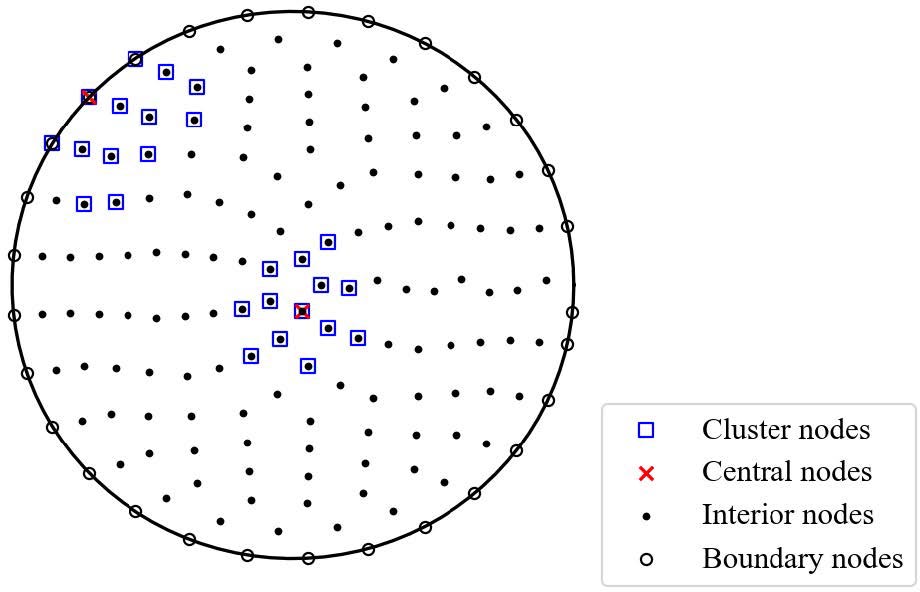
Figure 1: Schematic diagram of GFDM. Irrespectively of the position of the central node, being an interior or a boundary node, 12 suitably- chosen adjacent nodes constitute a point cluster.

The error between the expanded and actual values, the residual function, can be expressed as

$B(\phi )$	$={\displaystyle \sum _{i=1}^m}[({\phi }_0-{\phi }_i+h_i{\left({\displaystyle \frac{\partial \phi }{\partial x}}\right)}_0+k_i{\left({\displaystyle \frac{\partial \phi }{\partial y}}\right)}_0$
$\mathrm{\hspace{1em}}+{\displaystyle \frac{h_i^2}{2}}{\left({\displaystyle \frac{{\partial }^2\phi }{\partial x^2}}\right)}_0+{\displaystyle \frac{k_i^2}{2}}{\left({\displaystyle \frac{{\partial }^2\phi }{\partial y^2}}\right)}_0$
$\mathrm{\hspace{1em}}+h_i{k}_i{\left({\displaystyle \frac{{\partial }^2\phi }{\partial x\partial y}}\right)}_0)\omega ({\mathit{\text{X}}}_i)]{}^2,$	(3)

where $\omega ({\mathit{\text{X}}}_{\mathbf{i}})$ is the error weighting function. The expression of weighting function is not unique, but they all have a common feature, that is, the closer they are to center node, the greater the weight given, and the greater the contribution to the final calculation result. In this paper, the expression of $\omega ({\mathit{\text{X}}}_{\mathbf{i}})$ is defined as

$$\omega ({\mathit{\text{X}}}_{\mathbf{i}})=1-6{\left(\frac{d_i}{d_{\max }}\right)}^2+8{\left(\frac{d_i}{d_{\max }}\right)}^3-3{\left(\frac{d_i}{d_{\max }}\right)}^4,$$

(4)

where $d_i$ represents the distance from ${\mathit{\text{X}}}_{\mathbf{i}}$ to ${\mathit{\text{X}}}_{\mathbf{0}}$, and $d_{\max }$ is the maximum value among all $d_i$. The coefficient in $\omega ({\mathit{\text{X}}}_{\mathbf{i}})$ adds up to 0, which changes the function range from 0 to 1. In addition, the function $\omega ({\mathit{\text{X}}}_{\mathbf{i}})$ is monotonically decreasing and has a pole when $d_i/d_{\max }$ equals 0 or 1, which makes the function smooth. This construction also implies that $\omega ({\mathit{\text{X}}}_{\mathbf{i}})$ decreases rapidly when $d_i$ increases, which explicitly gives the weight distribution of each point in the cluster.

For brevity, define

$${\mathbf{D}}_{\phi }={[\frac{\partial \phi }{\partial x},\frac{\partial \phi }{\partial y},\frac{{\partial }^2\phi }{\partial x^2},\frac{{\partial }^2\phi }{\partial y^2},\frac{{\partial }^2\phi }{\partial x\partial y}]}^T,$$

(5)

$$p_i=\{h_i,k_i,\frac{h_i^2}{2},\frac{k_i^2}{2},h_i{k}_i\},$$

(6)

$$\mathbf{P}=\left[\begin{array}{c}\hfill \begin{array}{c}\hfill p_1\hfill \\ \hfill p_2\hfill \end{array}\hfill \\ \hfill \begin{array}{c}\hfill \mathrm{⋮}\hfill \\ \hfill p_m\hfill \end{array}\hfill \end{array}\right]=\left[\begin{array}{cc}\hfill \begin{array}{cc}\hfill h_1\hfill & \hfill k_1\hfill \\ \hfill h_2\hfill & \hfill k_2\hfill \end{array}\hfill & \hfill \begin{array}{cc}\hfill \mathrm{\cdots }\hfill & \hfill h_1{k}_1\hfill \\ \hfill \mathrm{\cdots }\hfill & \hfill h_2{k}_2\hfill \end{array}\hfill \\ \hfill \begin{array}{cc}\hfill \mathrm{⋮}\hfill & \hfill \mathrm{⋮}\hfill \\ \hfill h_m\hfill & \hfill k_m\hfill \end{array}\hfill & \hfill \begin{array}{cc}\hfill \mathrm{\ddots }\hfill & \hfill \mathrm{⋮}\hfill \\ \hfill \mathrm{\cdots }\hfill & \hfill h_m{k}_m\hfill \end{array}\hfill \end{array}\right].$$

(7)

Then the residual function $B\left(\phi \right)$ in eqn (2.1) can be expressed in the form of the matrix as

$$\text{B}\left(\phi \right)={\left({\mathbf{PD}}_{\phi }+{\mathbf{\Phi }}_0-\mathbf{\Phi }\right)}^T\mathbf{W}\left({\mathbf{PD}}_{\phi }+{\mathbf{\Phi }}_0-\mathbf{\Phi }\right),$$

(8)

where $\mathbf{\Phi }={[{\phi }_1,\mathrm{\dots },{\phi }_m]}^T$ and ${\mathbf{\Phi }}_0$=${[{\phi }_0,\mathrm{\dots },{\phi }_0]}^T$ are the vectors of function values sampled at ${\mathit{\text{X}}}_{\mathbf{i}}$ and ${\mathit{\text{X}}}_{\mathbf{0}}$, respectively. Furthermore, $\mathbf{W}=\mathrm{diag}({\omega }_1^2,\mathrm{\dots },{\omega }_m^2)$ is a diagonal matrix.

The residual function can be regarded as a cost function in an optimization algorithm with the elements in $D_{\phi }$ as independent variables. The optimal solution is obtained by minimizing the norm $B\left(\phi \right)$

$$\frac{\partial B}{\partial \left\{{\mathit{\text{D}}}_{\phi }\right\}}=0,$$

(9)

resulting in the linear equation

$${\mathbf{AD}}_{\phi }=\mathbf{b},$$

(10)

with $\mathbf{A}={\mathbf{P}}^T\mathbf{WP}$ and $\mathbf{b}={\mathbf{P}}^T\mathbf{W}\left(\mathbf{\Phi }-{\mathbf{\Phi }}_0\right)$. The matrix $\mathbf{A}$ is symmetric, and, thus, the Cholesky decomposition method can be used to solve eqn (10). The expression of $\mathbf{A}$ indicates that at least five adjacent nodes should be found to construct the difference scheme; otherwise, the matrix $\mathbf{A}$ is not invertible because its rank must satisfy the condition: $\mathrm{rank}(\mathbf{A})=\min \{\mathrm{rank}\left(\mathbf{P}\right),\mathrm{rank}\left(\mathbf{W}\right)\}$.

By solving eqn (10), ${\mathbf{D}}_{\phi }$ can be expressed as

$${\mathbf{D}}_{\phi }={\mathbf{A}}^{-1}(-\sum _{i=1}^m{\omega }_i^2{p}_i^T,{\omega }_1^2{p}_1^T,\mathrm{\dots },{\omega }_m^2{p}_m^T)\left(\begin{array}{c}\hfill \begin{array}{c}\hfill {\varphi }_0\hfill \\ \hfill {\varphi }_1\hfill \end{array}\hfill \\ \hfill \begin{array}{c}\hfill \mathrm{⋮}\hfill \\ \hfill {\varphi }_m\hfill \end{array}\hfill \end{array}\right).$$

(11)

Eqn (11) shows that all second-order derivatives at center node ${\mathit{\text{X}}}_{\mathbf{0}}$ can be represented by a linear combination of function values at the nodes in point cluster. Each row element of the coefficient matrix in front of the vector ${[{\phi }_0,{\phi }_1,\mathrm{\dots },{\phi }_0]}^{\mathrm{T}}$corresponds to the difference result of each element in ${\mathbf{D}}_{\phi }$.

B. Improved version of GFDM

From the above difference scheme, it can be seen that at least five adjacent nodes need to be found to represent the derivative at center node, which provides an idea for the improved version of GFDM. The second derivative of $\phi (\mathit{\text{X}})$ with respect to each variable of $x$ and $y$ at the node ${\mathit{\text{X}}}_{\mathbf{0}}$ is approximated as linear combinations of the neighbor nodes

$$L\phi \left({\mathit{\text{X}}}_{\mathbf{0}}\right)=\sum _{i=0}^5{c}_i{\phi }_i,$$

(12)

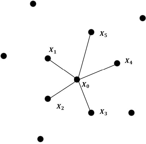
Figure 2: Schematic diagram of improved version of GFDM. Only five adjacent nodes around the central node need to be found to construct a point cluster.

where $L$ represents the derivative operator of the governing equation that $\phi$ satisfies, and $c_i,i=0,\mathrm{\dots },5$ are weight coefficients to be determined. First, expand these five nodes according to eqn (2.1) and then group similar terms. According to the coefficient in front of the similar term and the corresponding coefficient in $L$ are strictly equal, the following matrix equation can beobtained:

$$\left[\begin{array}{cccccc}\hfill 1\hfill & \hfill 1\hfill & \hfill 1\hfill & \hfill 1\hfill & \hfill 1\hfill & \hfill 1\hfill \\ \hfill 0\hfill & \hfill h_1\hfill & \hfill h_2\hfill & \hfill h_3\hfill & \hfill h_4\hfill & \hfill h_5\hfill \\ \hfill 0\hfill & \hfill k_1\hfill & \hfill k_2\hfill & \hfill k_3\hfill & \hfill k_4\hfill & \hfill k_5\hfill \\ \hfill 0\hfill & \hfill h_1^2/2\hfill & \hfill h_2^2/2\hfill & \hfill h_3^2/2\hfill & \hfill h_4^2/2\hfill & \hfill h_5^2/2\hfill \\ \hfill 0\hfill & \hfill k_1^2/2\hfill & \hfill k_2^2/2\hfill & \hfill k_3^2/2\hfill & \hfill k_4^2/2\hfill & \hfill k_5^2/2\hfill \\ \hfill 0\hfill & \hfill h_1{k}_1\hfill & \hfill h_2{k}_2\hfill & \hfill h_3{k}_3\hfill & \hfill h_4{k}_4\hfill & \hfill h_5{k}_5\hfill \end{array}\right]\left[\begin{array}{c}\hfill c_0\hfill \\ \hfill c_1\hfill \\ \hfill c_2\hfill \\ \hfill c_3\hfill \\ \hfill c_4\hfill \\ \hfill c_5\hfill \end{array}\right]=\left[\begin{array}{c}\hfill b_0\hfill \\ \hfill b_1\hfill \\ \hfill b_2\hfill \\ \hfill b_3\hfill \\ \hfill b_4\hfill \\ \hfill b_5\hfill \end{array}\right],$$

(13)

where $b_0$ is the coefficient in front of ${\phi }_0$, $b_i,i=1,\mathrm{\dots },5$ are the coefficients in front of each element in ${\mathbf{D}}_{\phi }$. The value of $b_i$ is determined by the governing equation. For example, when solving eqn (2.1), $b_i$ is the corresponding value in the set $\{0,{\lambda }_{10},{\lambda }_{01},{\lambda }_{20},{\lambda }_{02},{\lambda }_{11}\}$. The weight coefficient $c_i$ can be obtained by solving the matrix equation $\mathbf{Ac}=\mathbf{b}$ given by eqn (13).

When constructing a cluster of nodes around the boundary, several nodes on the boundary are also included. Assume that ${\mathit{\text{X}}}_{\mathbf{5}}$ is the boundary node and $\phi \left({\mathit{\text{X}}}_5\right)$ satisfies the Neumann boundary condition. Express the derivative at ${\mathit{\text{X}}}_{\mathbf{0}}$ as

$$L\phi \left({\mathit{\text{X}}}_0\right)=\sum _{i=0}^4{c}_i{\phi }_i+c_5\overline{r}{\left(\frac{\partial \phi }{\partial n}\right)}_5.$$

(14)

Here, $\overline{r}$ is the average distance between adjacent nodes and the center nodes. The purpose of adding this item is to ensure that all coefficients are in the same order of magnitude. Expand the last term in eqn (14) according to Taylor’s series formula

${\left({\displaystyle \frac{\partial \phi }{\partial n}}\right)}_0=$	${\left({\displaystyle \frac{\partial \phi }{\partial x}}\right)}_0{n}_x+{\left({\displaystyle \frac{\partial \phi }{\partial y}}\right)}_0{n}_y$
$+\left({\left({\displaystyle \frac{{\partial }^2\phi }{\partial x^2}}\right)}_0{n}_x+{\left({\displaystyle \frac{{\partial }^2\phi }{\partial x\partial y}}\right)}_0{n}_y\right)h_5$
$+\left({\left({\displaystyle \frac{{\partial }^2\phi }{\partial x\partial y}}\right)}_0{n}_x+{\left({\displaystyle \frac{{\partial }^2\phi }{\partial y^2}}\right)}_0{n}_y\right)k_5,$	(15)

where $n_x$ and $n_y$ correspond to the axial component of the unit normal vector at node ${\mathit{\text{X}}}_{\mathbf{5}}$, respectively.

For each adjacent node, if it is located on the boundary, expand according to eqn (2.2); otherwise, it is expanded by eqn (2.1). Grouping terms of similar kind, the following matrix equation can be obtained:

$$\begin{array}{c}\hfill \left[\begin{array}{cccccc}\hfill 1\hfill & \hfill 1\hfill & \hfill 1\hfill & \hfill 1\hfill & \hfill 1\hfill & \hfill 0\hfill \\ \hfill 0\hfill & \hfill h_1\hfill & \hfill h_2\hfill & \hfill h_3\hfill & \hfill h_4\hfill & \hfill \overline{r}{n}_x\hfill \\ \hfill 0\hfill & \hfill k_1\hfill & \hfill k_2\hfill & \hfill k_3\hfill & \hfill k_4\hfill & \hfill \overline{r}{n}_y\hfill \\ \hfill 0\hfill & \hfill h_1^2/2\hfill & \hfill h_2^2/2\hfill & \hfill h_3^2/2\hfill & \hfill h_4^2/2\hfill & \hfill \overline{r}{n}_x{h}_5\hfill \\ \hfill 0\hfill & \hfill k_1^2/2\hfill & \hfill k_2^2/2\hfill & \hfill k_3^2/2\hfill & \hfill k_4^2/2\hfill & \hfill \overline{r}{n}_y{k}_5\hfill \\ \hfill 0\hfill & \hfill h_1{k}_1\hfill & \hfill h_2{k}_2\hfill & \hfill h_3{k}_3\hfill & \hfill h_4{k}_4\hfill & \hfill \overline{r}(n_y{h}_5+n_x{k}_5)\hfill \end{array}\right]\left[\begin{array}{c}\hfill c_0\hfill \\ \hfill c_1\hfill \\ \hfill c_2\hfill \\ \hfill c_3\hfill \\ \hfill c_4\hfill \\ \hfill c_5\hfill \end{array}\right]=\left[\begin{array}{c}\hfill b_0\hfill \\ \hfill b_1\hfill \\ \hfill b_2\hfill \\ \hfill b_3\hfill \\ \hfill b_4\hfill \\ \hfill b_5\hfill \end{array}\right]\end{array}.$$

(16)

The matrix markedasmathA in eqn (13) or eqn (16) must be automatically scaled by “1”, “$\overline{r}$”, and “${\overline{r}}^2$” because of the appearance of the first and second derivatives. Vector markedasmathb has to make the same change to ensure the equation is correct. In addition, taking $\overline{r}$ as a normalized factor can effectively avoid the singularity of matrix due to uneven distribution of adjacent points.

C. General steps for analyzing waveguides

When electromagnetic waves propagate in a uniform metal waveguide with the axis along the z-direction, the governing equations and boundary conditions that the electromagnetic field satisfies are

$$L\phi +k_c^2\phi =0$$

(17)

$$L_B\phi =0,$$

(18)

where $\phi$ is the electromagnetic field component, $k_c$ is the cutoff wavenumber, $L={\nabla }_t^2$ is the transverse Laplacian operator, and $L_B$ is the boundary operator. When propagating TM wave, $\phi =E_z$, $L_B$ refers to the Dirichlet boundary $E_z=0$. When propagating TE wave, $\phi =H_z$, $L_B$ refers to the Neumann boundary $\partial H_z/\partial n=0$.

As the generalized finite difference scheme given by eqn (11), GFDM simultaneously gives the numerical discrete results of all derivatives of $\phi \left(\mathit{\text{X}}\right)$ at a certain node; so the coefficient matrix obtained by GFDM should be combined according to the governing equation. The difference result of the internal node is multiplied by the vector $[0,0,1,1,0]$ because it satisfies the Laplace equation. For nodes on the boundary, when solving the TM wave problem, the differential processing is not required because the boundary value $\phi =0$ is known, and when solving the TE wave problem, the result should be multiplied by the vector $[n_x,n_y,0,0,0]$ because the Neumann boundary condition is satisfied.

First, we arrange $N_I$ discrete points inside the cross section and $N_B$ discrete points on the boundary, with $N=N_I+N_B$. According to the difference scheme for solving the waveguide problem given above, the internal node repeats this process $N_I$ times to obtain the matrix $A$, and eqn (17) can be written as

$$\left[\begin{array}{cc}\hfill {\mathit{\text{A}}}_{\mathit{\text{I}}}\hfill & \hfill {\mathit{\text{A}}}_{\mathit{\text{B}}}\hfill \end{array}\right]\left[\begin{array}{c}\hfill {\mathit{\phi }}_{\mathit{\text{I}}}\hfill \\ \hfill {\mathit{\phi }}_{\mathit{\text{B}}}\hfill \end{array}\right]=-{\mathit{\text{k}}}_{\mathbf{c}}^{\mathbf{2}}{\mathit{\phi }}_{\mathit{\text{I}}},$$

(19)

where ${\mathit{\phi }}_I={[{\phi }_1,\mathrm{\dots },{\phi }_{N_I}]}^{\mathrm{T}}\mathrm{and}{\mathit{\phi }}_B={[{\phi }_{N_I+1},\mathrm{\dots },{\phi }_N]}^{\mathrm{T}}$. For nodes on the boundary, when Neumann BCs have to be satisfied, matrix B can be obtained similarly

$$\left[\begin{array}{cc}\hfill {\mathit{\text{B}}}_I\hfill & \hfill {\mathit{\text{B}}}_B\hfill \end{array}\right]\left[\begin{array}{c}\hfill {\mathit{\phi }}_{\mathit{\text{I}}}\hfill \\ \hfill {\mathit{\phi }}_{\mathit{\text{B}}}\hfill \end{array}\right]=\mathbf{0}.$$

(20)

Combining eqn (19) and (20), the eigenvalue equation describing the waveguide problem can be discretized and written in the matrix form

$$\left[\begin{array}{cc}\hfill {\mathit{\text{A}}}_I\hfill & \hfill -{\mathit{\text{A}}}_{\mathit{\text{B}}}\left({\mathit{\text{B}}}_{\mathit{\text{B}}}^{-1}{\mathit{\text{B}}}_I\right)\hfill \end{array}\right]{\mathit{\phi }}_I=-k_c^2{\mathit{\phi }}_I.$$

(21)

The Dirichlet boundary condition can be directly substituted into the matrix because ${\mathit{\phi }}_{\mathit{\text{B}}}=\mathbf{0}$ means that the weight coefficients of the boundary nodes in the generalized finite difference schema can be ignored, that is, the matrix ${\mathit{\text{A}}}_{\mathit{\text{B}}}$ can be omitted.

When using the improved version of GFDM to solve the waveguide problem, the value of vector $b$ is $[0,0,0,1,1,0]$. Compared with traditional GFDM, the coefficient matrix can be constructed more conveniently by eqn (13) and (16). Especially when solving the TE wave problem, the boundary node avoids additional differencing because the Neumann boundary can be directly used as shown in eqn (14).

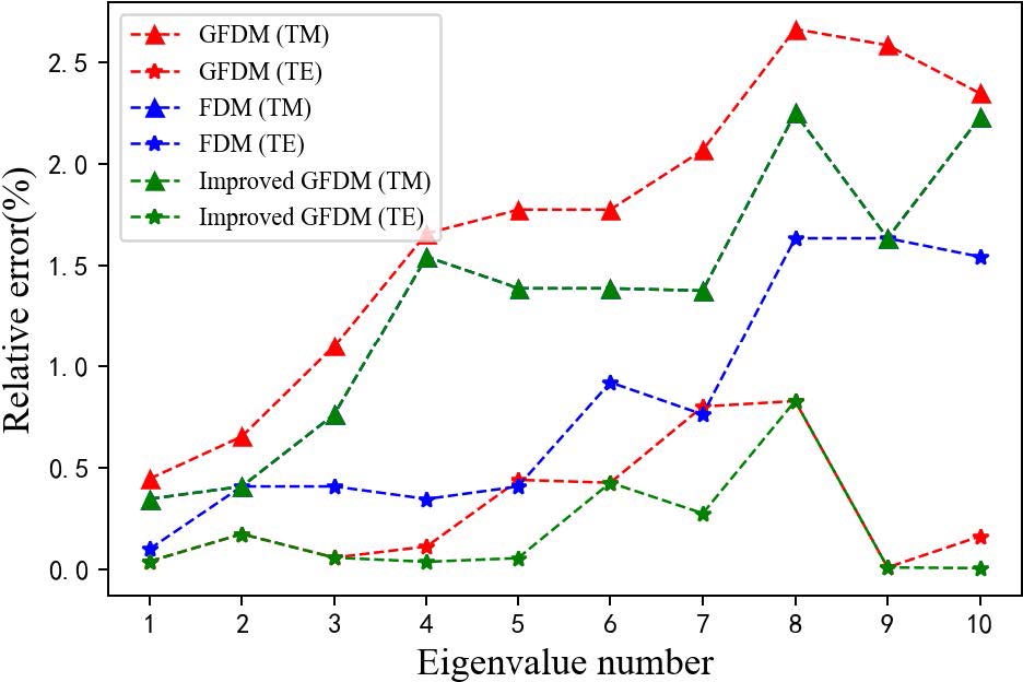
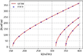
Figure 3: Error comparison of GFDM solution, FDM solution, and improved GFDM solution for cutoff wavenumbers of the TM wave and TE wave in the rectangular waveguide. The “improved GFDM (TM)” line and the “FDM (TM)” line coincide.

III. NUMERICAL RESULTS

To validate the GFDM in analyzing the waveguide eigenvalue problems, we analyzed the dispersion characteristics of TE modes and TM modes in different waveguides. The size of the point cluster in GFDM is set to be 10. The GFDM solution is compared with the FDM, FDFD, and RBF solutions, and the reasons for the differences in the result are also given.

First, we consider a rectangular waveguide with a size of $20\mathrm{mm}\times 10\mathrm{mm}$ and divide the calculation domain uniformly at intervals of $1\mathrm{mm}$. Figure 3 shows the error comparison of GFDM solution, FDM solution, and improved GFDM solution for cutoff wavenumbers of the TM wave and TE wave in the rectangular waveguide. When solving TM wave problems, the improved GFDM solution is equal to the FDM solution because the equally spaced and uniform distribution of the sampling points leads to the same weight coefficient obtained by eqn (13) as the FDM. When solving TE wave problems, the improved GFDM and GFDM have obvious advantages over FDM by virtue of the handing of Neumann boundary conditions. This is because FDM needs an extra layer of grid outside the boundary in order to deal with the Neumann BCs, and the value of these grids is equal to the function value of the nodes symmetrical to it in the boundary. This means that the nodes on the boundary must also be differentiated according to the governing equation, and this process produces additional errors. In addition, FDM needs to modify the difference formula to satisfy the boundary conditions, while the solution process of GFDM is more versatile.

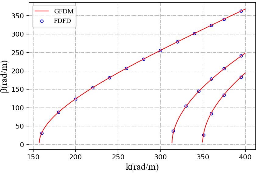
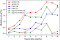
Figure 4: Dispersion characteristics of $T{E}_{10}$, $T{E}_{01}$, and $T{M}_{11}$ modes in rectangular waveguide. Results are calculated using GFDM and FDFD.

Figure 4 shows the dispersion characteristics of ${\mathrm{TE}}_{10},{\mathrm{TE}}_{01}$, and ${\mathrm{TM}}_{11}$ modes in rectangular waveguide by using GFDM and FDFD, respectively. The improved GFDM is not included in Figure 4 because it is almost equal to the GFDM solution, which can be seen from Figure 1. The eigenvalue equation of FDFD is derived from Maxwell’s curl equations, where the eigenvalue and eigenvector expressions are $\beta /k_0$ and ${[E_x,E_y,H_x,H_y]}^{\mathrm{T}}$, respectively. This method cannot directly yield $k_c$ for each mode, nor can it determine the wave transmission mode; so the results are given as scatter points. Since the eigenvector involves four field components, the correction of the FDFD difference formula at the boundary is more complicated than that of FDM, and it is necessary to consider both the Dirichlet BCs and the Neumann BCs. In addition, each discrete point of FDFD will produce two variables. Consequently, the size of the coefficient matrix obtained by FDFD is about $2N_I\times 2N_I$, and the size of GFDM is about $N_I\times N_I$. This means that using the same subdivision, GFDM saves memory space when compared against FDFD.

RBF is similar to GFDM, and both express the derivative at the center node by the weighted sum of the function values of each node in the point cluster. The size of the point cluster $N_s$ in RBF needs to satisfy $N_s\gtrsim 2N_p$, where $N_p$ is the number of polynomials included in the interpolation function, and the value of $N_p$ is related to the highest degree $d$ of the polynomial. For example, when $d$= 2, all polynomials are $\{1,x,y,x^2,y^2,xy\}$, the number of polynomials is $N_p=6$, and RBF requires that the cluster size must satisfy $N_s\gtrsim 12$.

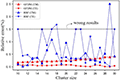
Take a circular waveguide with a radius of $1\mathrm{mm}$ as an example to compare the stability and accuracy of GFDM and RBF. The numbers of computational points inside the cross section and on the boundary are $N_I=305\mathit{\hspace{1em}}\mathrm{and}{N}_B=50$, and the cluster size is set to be 12. Figure 5 shows the relative error of the GFDM solution and RBF solution of the TE main mode and TM main mode in circular waveguide at different cluster sizes. If the relative error in the figure is on the dotted line, it means that the result is wrong. The improved GFDM result was not used for comparison because its cluster size was fixed to be 6. As the point cluster size changes, GFDM is significantly more stable and accurate than RBF. It is worth mentioning that although increasing the number of polynomials in RBF is beneficial to improving the performance of the method, it means that more adjacent nodes need to be found to represent the derivative, which will lead to a sharp increase in the amount of calculation. Table 1 gives the comparison of computer execution time between GFDM and RBF under the same sampling point and cluster size. As the number of adjacent points increases, that is, the size of the point cluster increases, the advantages of GFDM are more obvious. The main reason is that RBF needs to calculate the distance between each node in the point cluster and all remaining nodes, when calculating the weight coefficient, while GFDM only requires the distance between the central node and the adjacent nodes.

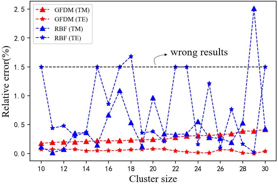
Figure 5: Error comparison between the GFDM solution and the RBF solution of the cutoff wavenumbers of the TE main mode and TM main mode in the circular waveguide.

Table 1: Comparison of computer execution time in GFDM and RBF

Point cluster size	GFDM	RBF
12	0.3886 s	0.7555 s
20	0.4080 s	1.5053 s
30	0.4333 s	2.8191 s

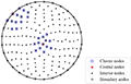
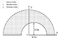
Figure 6: The distribution of computational nodes on the cross-section of the eccentric circular waveguide when solving even TM modes. The outer and inner radii of the waveguide are a and 0.5a, respectively. The distance between the two circle centers is 0.2a.

Table 2: Normalized cutoff wavenumber for the first six even TM modes

Traditional GFDM	Improved GFDM	Method in [5]
4.8001	4.8016	4.8106
6.1505	6.1530	6.1724
7.3591	7.3646	7.3945
8.4473	8.4591	8.4974
9.2701	9.2776	9.3409
9.4048	9.4198	9.4739

Finally, GFDM and an improved version of GFDM are used to solve the cutoff wavenumbers of an eccentric circular waveguide. Since the cross section of the waveguide is symmetrical about the x-axis, the odd and even modes can be solved separately. Figure 6 shows the distribution of computational nodes on the cross section of the eccentric circular waveguide when solving even TM modes. As shown in Table 2, the results of traditional GFDM and improved GFDM agree with the results given in [5].

IV. CONCLUSION

In this paper, the effectiveness of GFDM to solve the eigenvalue problem for the waveguide is verified. Compared with FDM and FDFD, GFDM avoids the complicated meshing process, and the difference formula is more versatile. What is more, GFDM owns the meshless feature to better handle Neumann boundary conditions. Compared with RBF, which is one of the meshless methods, GFDM has higher efficiency and better stability. GFDM provides a new idea and contributes significantly to solving the eigenvalue problems associated with waveguides.

V. ACKNOWLEDGMENT

This work was supported in part by the NUPTSF under Grant NY220074, by the National Nature Science Foundation of China for Youth under Grant 62001245, by the Natural Science Foundation of Jiangsu Province for Youth under Grant BK20200757, and by the State Key Laboratory of Millimeter Waves under Grant K202108. The authors are grateful to Prof. Ming Zhang for the useful discussions.

REFERENCES

[1] J. R. Pyle, “The cutoff wavelength of the ${\mathrm{TE}}_{10}$ mode in ridged rectangular waveguide of any aspect ratio,” IEEE Trans. Microw. Theory and Techn., vol. 14, no. 4, pp. 175-183, Apr. 1966.

[2] Y. J. Zhao, K. L. Wu, and K. Cheng, “A compact 2-D full-wave finite-difference frequency-domain method for general guided wave structures,” IEEE Trans. Microw. Theory and Techn., vol. 50, no. 7, pp. 1844-1848, Jul. 2002.

[3] D. H. Chai, Harrington, and W. Hoefer, “The Finite-Difference-Time-Domain method and its application to eigenvalue problems,” IEEE Trans. Microw. Theory and Techn., vo. 34, no. 12, pp. 1464-1470, Dec. 1986.

[4] J. Svedin, “Propagation analysis of chirowaveguides using the finite-element method,” IEEE Trans. Microw. Theory and Techn., vol. 38, no. 10, pp. 1488-1496, Oct. 1990.

[5] J. A. Pereda and A. Grande, “Analysis of homogeneous waveguides via the meshless radial basis Function-Generated-Finite-Difference method,” IEEE Micro. and Wirel. Compon. Lett., vol. 30, no. 3, pp. 229-232, Mar. 2020.

[6] V. Lombardi, M. Bozzi, and L. Perregrini, “Evaluation of the dispersion diagram of inhomogeneous waveguides by the variational meshless method,” IEEE Trans. Microw. Theory and Techn., vol. 67, no. 6, pp. 2105-2113, Jun. 2019.

[7] S. Yang, Z. Chen, and Y. Yu, “A Divergence-Free meshless method based on the vector basis function for transient electromagnetic analysis,” IEEE Trans. Microw. Theory and Techn., vol. 62, no. 7, pp. 1409-1416, Jul. 2014.

[8] L. Gavete, M. L. Gavete, and J. J. Benito, “Improvements of generalized finite difference method and comparison with other meshless method,” Appl. Math. Model., vol. 27, no. 10, pp. 831-847, Oct. 2003.

[9] L. Gavete, F. Urena, and J. J. Benito, “Solving second order non-linear elliptic partial differential equations using generalized finite difference method,” J. Comput. Appl. Math., vol. 318,pp. 378-387, Jul. 2017.

[10] J. J. Benito, and F. Urea, “An h-adaptive method in the generalized finite differences,” Comput. Meth. Appl. Mech. Eng., vol. 192, no. 5-6, pp. 735-759, Jan. 2003.

[11] J. J. Benito, F. Urena, and L. Gavete, “Influence of several factors in the generalized finite difference method,” Appl. Math. Model., vol. 25, no. 12, pp. 1039-1053, Dec. 2001.

[12] A. Kamyabi, V. Kermani, and M. Kamyabi, “Improvements to the meshless generalized finite difference method,” Eng. Anal. Bound. Elem., vol. 99, pp. 233-243, Feb. 2019.

[13] P. W. Li and C. M. Fan, “Generalized finite difference method for two-dimensional shallow water equations,” Eng. Anal. Bound. Elem., vol. 80, pp. 58-71, Jul. 2017.

[14] Y. Gu and L. Wang, “Application of the meshless generalized finite difference method to inverse heat source problems,” Int. J. Heat Mass Transf., vol. 108, pp. 721-729, May 2017.

[15] T. Zhang, Y. F. Ren, C. M. Fan, and P. W. Li, “Simulation of two-dimensional sloshing phenomenon by generalized finite difference method,” Eng. Anal. Bound. Elem., vol. 63, pp. 82-91,Feb. 2016.

[16] C. Jian, G. Yan, and M. Wang, “Application of the generalized finite difference method to three-dimensional transient electromagnetic problems,” Eng. Anal. Bound. Elem., vol. 92, pp. 257-266, Jul. 2017.

[17] H. Xu, Y. C. Mei, and Y. Bao, “Application of generalized finite difference method in analysis of transmission characteristics of waveguide,” 2020 APMC., Hong Kong., China, pp. 785-787, 2020.

BIOGRAPHIES

Hui Xu was born in Wuxi, Jiangsu, China. He received the B.Eng. degree from the Nanjing University of Posts and Telecommunications, Nanjing, China. He is currently working toward the M.S. degree with the School of Electronic and Optical Engineering, Nanjing University of Posts and Telecommunications.

His research interests include the electromagnetic field theory, electromagnetic engineering, and computer aided analysis and design.

Yang Bao was born in Nanjing, Jiangsu, China. He received the B.Eng. and M.S. degrees from the Nanjing University of Posts and Telecommunications, Nanjing, China, in 2011 and 2014, respectively, and the Ph.D. degree in electrical engineering from Iowa State University, Ames, IA, USA, in 2019.

In December 2019, he joined the Nanjing University of Posts and Telecommunications as an Assistant Professor with the School of Electronic and Optical Engineering. His research interests focus on modeling and simulations of composite material, electromagnetic wave scattering using fast algorithms, and eddy current nondestructive evaluation.

ACES JOURNAL, Vol. 37, No. 3, 266–272.
doi: 10.13052/2022.ACES.J.370302
© 2021 River Publishers

Abstract

I. INTRODUCTION

II. FORMULATION OF GFDM

A. Basic theory of GFDM

B. Improved version of GFDM

C. General steps for analyzing waveguides

III. NUMERICAL RESULTS

IV. CONCLUSION

V. ACKNOWLEDGMENT

REFERENCES

BIOGRAPHIES