3D Dynamic Ray-tracing Propagation Model with Moving Scatterer Effects
Gang Liu, Tao Wei, and Chong-Hu Cheng
1College of Physics and Electronic Engineering Taishan University, Tai’an 271000, China
gd0713liugang@163.com
2College of Electronic and Optical Engineering & College of Microelectronics, Nanjing University of Posts and Telecommunications, Nanjing 210023, China
taotaotao110@163.com, chengch@njupt.edu.cn
Submitted On: November 2, 2021; Accepted On: May 8, 2022
Abstract
Ray-tracing propagation model (RTPM) has been widely used for predicting channel characteristics, whereas the scenarios considered are generally static. The complexity of RTPM is significantly increased due to the rapidly time-varying scenario resulted from moving scatterers. A three-dimensional (3D) dynamic RTPM considering moving scatterer effects is advanced in this paper. First, a simplified dynamic scenario preprocessing method based on the predefined active region and face transformation is proposed. The random movement of multiple scatterers can be enabled without repeated scenario modeling. Second, an efficient dynamic ray-tracing method based on self-adaptive ray-launching technique is advanced. The computational efficiency of the dynamic RTPM can be significantly improved due to the exclusion of repeated ray-tracing process over time. Finally, the feasibility and accuracy of the RTPM is verified by comparing the simulation results with the measurements performed in an indoor scenario with pedestrians.
Keywords: Dynamic ray-tracing, moving scatterers, self-adaptive ray-launching technique.
I. INTRODUCTION
Dynamic scenarios (e.g., shopping mall, waiting hall, intelligent transportation, and intelligent plant) with moving scatterers (e.g., vehicles, machines, and pedestrians) are considered as one of the most important application scenarios for the B5G and 6G wireless communication systems [1–3]. Accurately predicting the channel characteristics in these scenarios is fundamental and crucial for system design. As a high performance solution, ray-tracing propagation model (RTPM) has been widely used in the prediction of channel characteristics [4–6]. However, these RTPMs are generally focused on the scenarios considering only staticscatterers.
The research on the RTPM for dynamic scenarios with moving scatterers is still scarce. For a dynamic scenario with moving scatterers, the complexity of a RTPM is extremely increased and generally reflected in two aspects. The first one is the scenario preprocessing such as the dynamic and continuously temporal channel representation. This is because the scenario is required to be modeled repeatedly once the locations of scatterers are changed. The other one is that performing ray-tracing simulations at each discrete time instant is indeed computationally expensive. Several dynamic ray-tracing models with the movement of transceiver are described in [7–9], whereas the moving scatterer effects are not considered. An image-visibility-based preprocessing method for dynamic ray tracing in urban environments is introduced in [10]. The dynamic visibility region is established according to the movement trajectory of the transmitter and scatterers. However, the trajectory is a priori and the dynamic visible region has to be reconstructed once trajectory is changed. Several efficient dynamic ray-tracing models considering moving scatterer effects are introduced in [11] and [12]. The efficiency of the dynamic ray-tracing models can be improved by replacing the simulation at each discrete time instant with single simulation in the coherent time. However, the coherent time for different scenarios is required to be obtained from a large number of measurements.
In this paper, a three-dimensional (3D) dynamic RTPM with moving scatterer effects is advanced. In view of the two problems that resulted from the moving scatterers as mentioned above, first, a simplified scenario preprocessing method is proposed. Based on the predefined active region and face transformation, scenario modeling and date processing are required to be performed only once in the entire dynamic ray-tracing process. Moreover, a self-adaptive ray-launching (SARL) based dynamic ray-tracing method is advanced to improve the computational efficiency by removing the redundant rays at each time instant.
II. 3D DYNAMIC RAY-TRACING PROPAGATION MODEL
In this section, a 3D dynamic RTPM is introduced from two aspects, including simplified dynamic scenario preprocessing and efficient dynamic ray-tracingmethod.
A. Simplified dynamic scenario preprocessing
Detailed scenario description such as the geometric structure and the layout of scatterers is necessary for RTPM. However, the random movement of scatterers leads to the real-time change of scenarios. Repeated scenario modeling and data processing result in the huge overhead of dynamic scenario preprocessing.
In order to simplify the dynamic scenario preprocessing, the static and moving scatterers are modeled independently. Static scatterers can be modeled according to the geometric structure and layout as same as the traditional RTPMs [13, 14]. However, for moving scatterers, an active region should be predefined according to the possible locations. Assuming that a moving scatterer can be modeled as a parallelepiped commonly used as one of the human and vehicle models [15, 16], the active region can be gridded as shown in Figure 1. All grids are required to be numbered without repetition and each grid is corresponding to a parallelepiped.
Second, space subdivision is performed to the whole scenario and the whole propagation space can be subdivided into many non-overlapping tetrahedrons. An instance of space subdivision for a room with a single scatterer is shown in Figure 2. Two types of faces are present in the scenario after space subdivision. The first one is called physical face (PF), i.e., the object surface. The PF property can be characterized by material parameters including the relative permittivity and the conductivity . The other one is called constructed face (CF). The faces are invisible and only used to assist the subsequent ray-tracing process. The material of CF is air and the corresponding parameters are and .
The appearance and disappearance of a scatterer can be modeled rapidly using a simple method of face property transformation (FPT). As shown in Figure 3, if all PF of a scatterer is transformed into CF (i.e., the forward FPT), rays pass through the scatterer without changing the propagation direction since CF has no effect on the rays. This indicates that the scatterer is equivalent to disappearing in the scenario. Conversely, if all CFs of the scatterer are converted into PF (i.e., the inverse FPT), the incident rays are interacted with the scatterer such as the reflection and diffraction. This indicates that the scatterer is equivalent to appearing in the scenario.
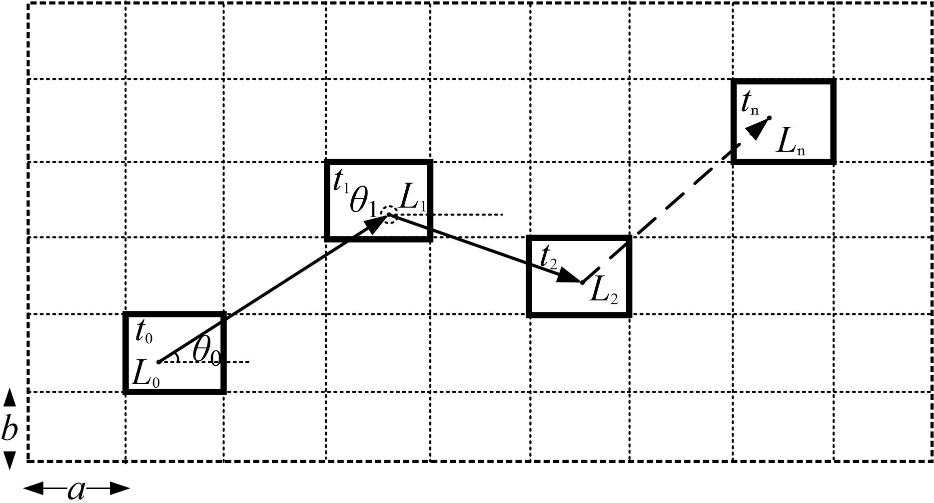
Figure 1: Random movement of a scatterer in a predefined activeregion.

Figure 2: An instance of space subdivision for a room with a single scatterer.
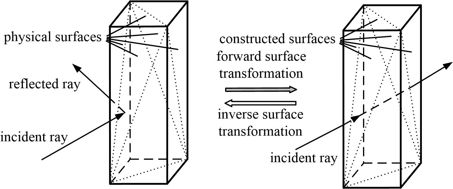
Figure 3: The appearance and disappearance fora moving scatterer using FPT.
The data of scenario after space subdivision can be stored in a tree structure with the depth of five as shown in Figure 4. The whole space of a scenario is assumed to be subdivided into T tetrahedrons on the second layer. Each tetrahedron corresponds to four faces stored in the third layer. The fourth layer is a crucial layer. In addition to three child nodes representing three lines, five leaf nodes are divided into three parts including two adjacent tetrahedrons related to the common face, the unit normal vector, and the face types, wherein the ray-object interaction mechanism can be determined according to the face types. The fifth layer is consisted of two parts, i.e., the two endpoints of each line and line types including constructed lines (CLs) and physical edges (PEs). As a result, the adjacent relationship between tetrahedrons can be obtained efficiently by traversing the tree structure.
B. Efficient dynamic ray-tracing method
The computational efficiency can be significantly reduced if performing ray-tracing process to all rays at each time instant. An SARL method is introduced to exclude the repeated ray-tracing process.
First, the forward FPT is applied to all parallelepipeds and this is equivalent to no moving scatterers in the scenario. As mentioned above, the propagation space has been subdivided into a number of tetrahedrons. A ray emitted from a transmitting point T can be intersected with a face of the tetrahedron containing T. The intersected face and the intersection point I can be determined as follows [17]:
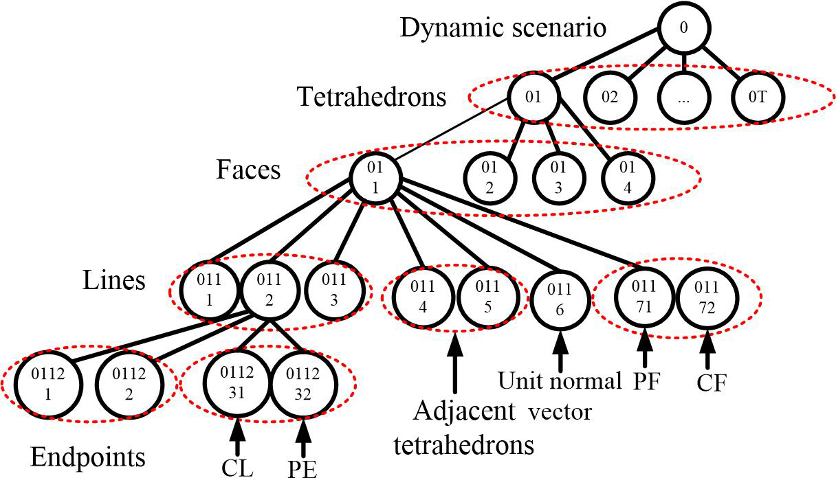
Figure 4: Data structure of scenario preprocessing.
| (1) |
| (2) |
where is the extension coefficient related to the i-th face. denotes the unit vector in the propagation direction. is the vector between T and one endpoint of the i-th face. is the unit normal vector of the i-th face. The intersected face is corresponding to the minimum and positive extension coefficient. If the intersected face is PF and the roughness is assumed to be neglected, the ray is reflected and the reflected field can be given as [18]
| (3) |
where is the attenuation coefficient and can be expressed as
| (4) |
where and d represent the distance from I to T and to a reference point on the reflected ray, respectively. The complex reflection coefficients for perpendicular and parallel polarizations are given as
| (5) |
| (6) |
where is the complex relative permittivity expressed as
| (7) |
where is the angular frequency and is the permittivity of vacuum.
Otherwise, if the intersected face is CF, the ray enters the adjacent tetrahedron without changing the propagation direction. Regardless of the intersected face being SF or CF, the intersection point I can be taken as the next transmitting point, and next intersection point can be determined from eqn (1) and (2). Consequently, the propagation path and received field of each ray can be determined.
In order to exclude the repeated ray-tracing process at each time instant, the sets of parallelepipeds intersected with rays are required to be recorded as
| (8) |
where s is the jth parallelepiped intersected with the k-th ray. K denotes the total number of rays. Consequently, the ray set corresponding to each parallelepiped can be also obtained and represented as
| (9) |
where r is the l-th ray related to the i-th parallelepiped. Q is the total number of parallelepipeds.
The dynamic RTPM can enable multiple scatterers to move independently and randomly. It is assumed that N moving scatterers are present in a scenario. At the initial time t, the initial locations of the N moving scatterers can be randomly generated from the grid indices and the N moving scatterers corresponding to the grids can be constructed based on the inverse FPT. The rays required to be retraced can be obtained from the set of scat_ray since only the paths of rays intersected with the N moving scatterers are changed. As a result, the total field can be determined as
| (10) |
where M and M denote the number of retained and retraced rays, respectively.
At time t, for the nth moving scatterer, a point can be randomly generated within the grid and taken as the start point . The speed v and direction angle can be generated according to the velocity models. For simplicity, assuming that the velocity is constant in the time interval (t-t), the velocity can be expressed as
| (11) |
where , , and denote the unit vectors of moving direction, x-axis direction, and y-axis direction, respectively. The reach point can be determined as
| (12) |
For multiple scatterers with different velocities, eqn (12) can be modified as
| (13) |
The grids containing the reach points represent the new locations of the N moving scatterers. The disappearance of moving scatterers at previous locations and the appearance of moving scatterers at new locations can be implemented using the forward and inverse FTP, respectively, and the scenario at time can be formed.
Similarly, the dynamic scenario with moving scatterers at each time instant can be determined. Furthermore, the total field at each time instant can be also obtained as eqn (10). Finally, the frame diagram of the 3D dynamic RTPM is shown in Figure 5. In view of the dynamic RTPM, the scenario modeling and space subdivision are required to be performed only once based on the predefined active region and FPT method, and, therefore, the dynamic scenario preprocessing can be significantly simplified. Moreover, only partial rays at each time instant are required to be retraced based on the SARL method and the efficiency of the dynamic ray-tracing process can be improved.
III. MODEL ANALYSIS
A. Scenario description
An indoor office scenario with pedestrians is considered in this paper. The size of the office is 7 m 6 m 2.5 m and the two-dimensional (2D) layout of the office with a predefined active region is shown in Figure 6. The office is composed of brick walls and the concrete ceiling and floor. There is no other furniture in the office except a wooden blackboard on the wall-D, a door on the wall-A, and a large glass window on the wall-B. Human body is modeled as a parallelepiped with the size of 0.3 m 0.3 m 1.7 m. The corresponding material parameters are listed in Table 1. The speed of pedestrians is assumed to be a constant of 0.5 m/s and pedestrians move from the left side to the right side of the office along a straight line. Vertically polarized omnidirectional antennas with the gain of 2.2 dBi are deployed at the transmitting and receiving sides. The transmitting antenna is 1.35 m above the floor level and 0.5 m from the wall-D. The frequency is 5.2 GHz and the transmitting power is 10 dBm. The height of receiving antenna is 0.85 m and the receiving antenna is 0.5 m from the wall-C.
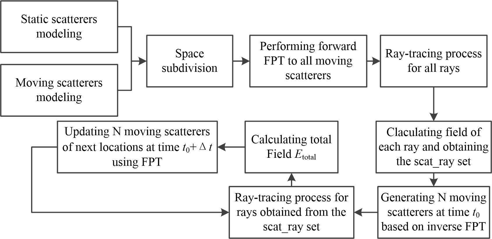
Figure 5: The frame diagram of the 3D dynamic ray-tracing propagation model.
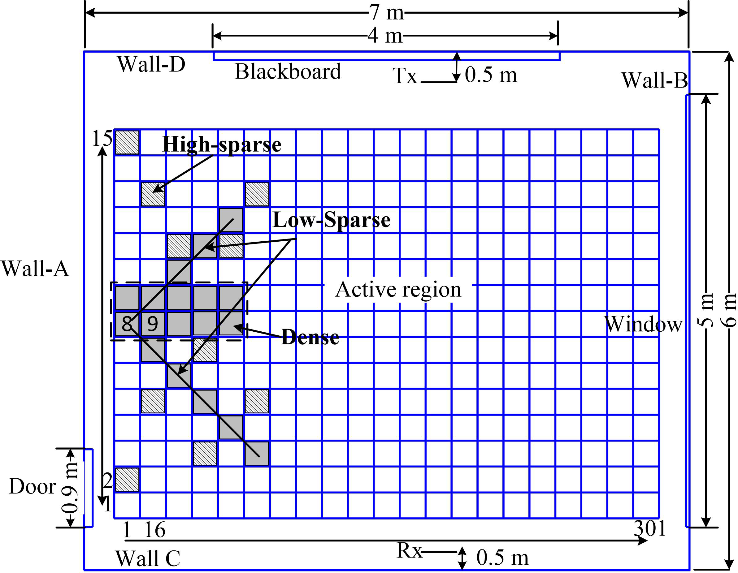
Figure 6: 2D layout of the office with a predefined active region.
Table 1: Material parameters
| Object | Relative permittivity |
Conductivity (S/m) |
|---|---|---|
| Brick wall | 4.0 | 0.343 |
| Concrete ceiling and floor | 6.14 | 1.005 |
| Glass window | 5.5 | 0.0 |
| Wooden blackboard | 2.1 | 0.05 |
| Human body | 38.5 | 2.4 |
B. Numerical results analysis
The received power can be expressed as [19]
| (14) |
where is the modulus operator. and denote the wavelength and the wave impedance in free space, respectively. G represents the receiving antenna gain. Considering a pedestrian (location 8 as shown in Figure 6) and two pedestrians (locations 8 and 9) move along a route perpendicular to the line between the transmitting and the receiving points. The time-varying received power is shown in Figures 7 and 8. The results show that the received power in the non-line-of-sight (NLOS) area is about 7 dB attenuation compared with the case of line-of-sight (LOS) due to the shadow effect of pedestrians. Furthermore, the received power for the scenario without pedestrians is also shown in Figure 8 as a reference. Up to 3 dB fluctuation of the received power compared with the case of empty room can be observed in the LOS area due to the multipath effect resulted from pedestrians. For the case of two pedestrians, a slightly offset in time is generated in the NLOS area. The simulation results show good agreement with the measurement results in [20] indicating the accuracy of the model.
In order to demonstrate the efficiency of the model, the simulation time of two dynamic RTPMs is investigated. The simulation has been carried out on a personal computer with the processor of Intel (R) core (TM) i5-7300hq CPU @ 2.50 GHz and the memory of 8 GB. The operating system is the 64-bit operating system of windows 10. Fortran computer language is used for the program implementation of the model and the running platform is Microsoft Visual Studio 2010. In the simulation, the total number of one hundred thousand source rays is traced at time t. The number of rays is a tradeoff between the computational accuracy and efficiency. For each time instant, the traditional ray-launching (RL) ray-tracing method is applied to all rays, whereas only the rays with changed paths are required to be retraced for the SARL ray-tracing method. The comparisons of simulation time between the traditional RL ray-tracing method and SARL ray-tracing method are listed in Table 2. Six dynamic scenarios considering different number of pedestrians (i.e., N = 2, 5, and 10) with multiple distributions (i.e., dense distribution, slight-sparsity distribution, and high-sparsity distribution) are considered.
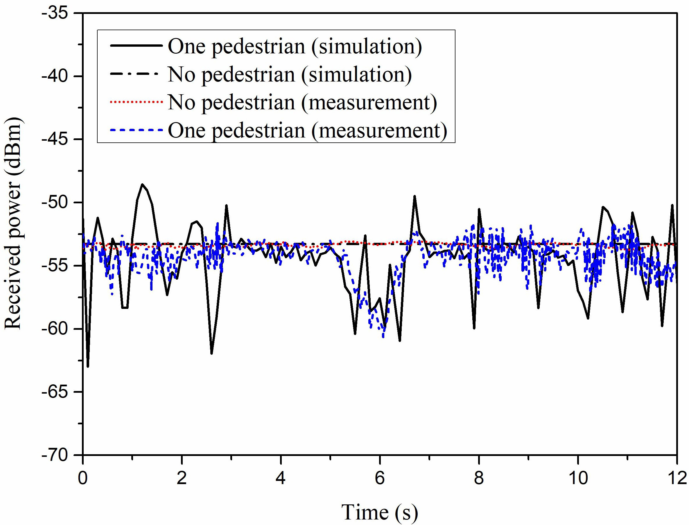
Figure 7: The time-varying received power for empty room and single pedestrian.
Table 2: Simulation time comparisons (unit: s)
| N | Method | Distribution | ||
| Dense | Low-sparsity | High-sparsity | ||
| 2 | RL | 72.8 | 73.12 | 72.7 |
| SARL | 7.69 | 8.48 | 8.18 | |
| 5 | RL | 73.6 | 74.6 | 75.1 |
| SARL | 9.2 | 9.61 | 9.67 | |
| 10 | RL | 74.1 | 76.6 | 76.6 |
| SARL | 9.63 | 11.14 | 11.27 |
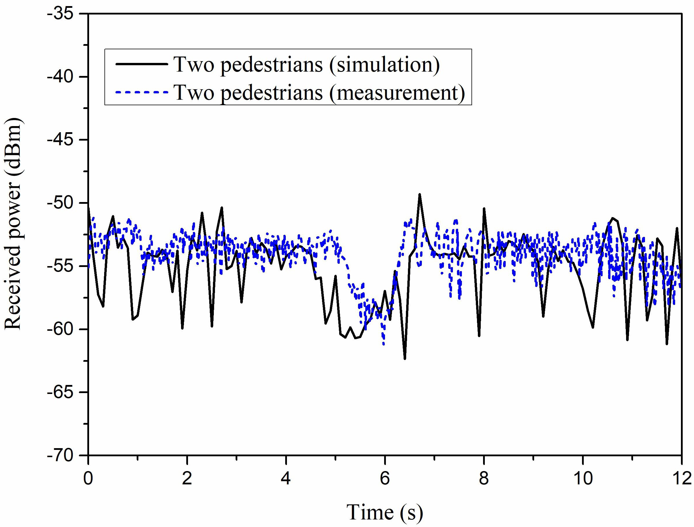
Figure 8: The time-varying received power for two pedestrians.
First, the results indicate that the simulation time is positively correlated with the number of pedestrians for two methods since the number of ray-object intersection tests is increased with the number of pedestrians. In addition, the paths of rays can be more readily changed with the increase of pedestrians. Second, more simulation time is required due to the increased dispersion degree of the distribution of moving scatterers. This is because the sparsely distributed scatterers lead to the paths of rays more likely to be changed especially for high-order reflection rays. Finally, the simulation time for RL is in the range of 72.7–76.6 s and is much higher than that for SARL in all scenarios due to the exclusion of repeated ray-tracing process. This indicates that the computational efficiency of dynamic ray-tracing model can be significantly improved using the SARL ray-tracing method.
IV. CONCLUSION
In this paper, an efficient 3D dynamic ray-tracing model has been advanced for the prediction of channel characteristics in the dynamic scenarios considering moving scatterers. In view of the moving scatterer effects on the increased complexity dynamic scenario preprocessing and reduced efficiency of ray-tracing process, first, a simplified dynamic scenario preprocessing method based on the predefined active region and FPT has been introduced. The simultaneous movement of multiple moving scatterers can be performed without repeated scenario modeling and date processing. Furthermore, an SARL-based dynamic ray-tracing method has been described. The repeated ray-tracing process can be eliminated at each time instant. The dynamic RTPM has been applied into an indoor office scenario considering multiple pedestrians and various distributions. The accuracy of the model has been verified by comparing the simulation results with the measurements. Furthermore, the reduced simulation time for SARL method compared with traditional RL method indicate that the computational efficiency of the proposed model can be significantly improved.
REFERENCES
[1] C. Wang, J. Huang, H. Wang, et al., “6G oriented wireless communication channel characteristics analysis and modeling,” Chinese Journal on Internet of Things, vol. 4, no. 1, 2020.
[2] B. Zong, C. Fan, X. Wang, et al., “6G technologies: Key drivers, core requirements, system architectures, and enabling technologies,” IEEE Vehicular Technology Magazine, vol. 14, no. 3, pp. 18-27, 2019.
[3] W. Saad, M. Bennis, and M. Chen, “A vision of 6G wireless systems: Applications, trends, technologies, and open research problems,” IEEE Network, vol. 34, no. 3, pp. 134-142, 2020.
[4] Z. Chen, H. Bertoni, and A. Delis, “Progressive and approximate techniques in ray-tracing based radio wave propagation prediction models,” IEEE Transactions on Antennas and Propagation, vol. 52, no. 1, pp. 240-251, 2004.
[5] Z. Q. Yun, and M. F. Iskander, “Ray tracing for radio propagation modeling: Principles and applications,” IEEE Access, vol. 3, pp. 1089-1100,2015.
[6] F. Fuschini, E. M. Vitucci, et al., “Ray tracing propagation modeling for future small-cell and indoor applications: A review of current techniques,” Radio Science, vol. 50, pp. 469-485, 2015.
[7] D. He, B. Ai, et al., “The design and applications of high-performance ray-tracing simulation platform for 5G and beyond wireless communications: A tutorial,” IEEE Communications Surveys & Tutorials, vol. 21, no. 1, pp. 10-27, 2019.
[8] L. Azpilicueta, C. Vargas-Rosales, and F. Falcone, “Intelligent vehicle communication: deterministic propagation prediction in transportation systems,” IEEE Vehicular Technology Magazine, vol. 11, no. 3, pp. 29-37, Sep. 2016.
[9] S. Hussain and C. Brennan, “Efficient preprocessed ray tracing for 5G mobile transmitter scenarios in urban microcellular environments,” IEEE Transactions on Antennas and Propagation, vol. 67, no. 5, pp. 3323-3333, May 2019.
[10] S. Hussain, and C. Brennan, “A dynamic visibility algorithm for ray tracing in outdoor environments with moving transmitters and scatterers,” IEEE 2020 14th European Conference on Antennas and Propagation, Copenhagen, Denmark, pp. 1-5, 2020.
[11] D. Bilibashi, E. M. Vitucci, and V. Degli-Esposti, “Dynamic ray tracing: Introduction and concept,” 2020 14th European Conference on Antennas and Propagation, Copenhagen, Denmark, pp. 1-5, 2020.
[12] F. Quatresooz, S. Demey, and C. Oestges, “Tracking of interaction points for improved dynamic ray tracing,” IEEE Transactions on Vehicular Technology, vol. 70, no. 7, pp. 6291-6301, Jul. 2021.
[13] G. E. Athanasiadou and A. R. Nix, “A novel 3-D indoor ray-tracing propagation model: The path generator and evaluation of narrow-band and wide-band predictions,” IEEE Transactions on Vehicular Technology, vol. 49, no. 7, pp. 1152-1168, 2000.
[14] S. Lored, L. Valle L, and R. P. Torres, “Accuracy analysis of GO/UTD radio-channel modeling in indoor scenarios at 1.8 and 2.5 GHz,” IEEE Antennas and Propagation Magazine, vol. 43, no. 5, pp. 37-51, 2001.
[15] M. Yang, Bo Ai, R He, et al., “Measurements and cluster-based modeling of vehicle-to-vehicle channels with large vehicle obstructions,” IEEE Transactions on Wireless Communications, vol. 19, no. 9, pp. 5860-5874, 2020.
[16] M. Mohamed, M. Cheffena, et al., “A dynamic channel model for indoor wireless signals: Working around interference caused by moving human bodies,” IEEE Antennas and Propagation Magazine, vol. 60, no. 2, pp. 82-91, 2018.
[17] G. Liu, J. She, W. Lu, et al., “3D deterministic ray tracing method for massive MIMO channel modelling and parameters extraction,” IET Communications, vol. 14, no. 18, pp. 3169-3174, 2020.
[18] H. R. Anderson, “A ray-tracing propagation model for digital broadcast systems in urban areas,” IEEE Transactions on Broadcasting, vol. 39, no. 3, pp. 309-317, 1993.
[19] A. Gifuni, “On the expression of the average power received by an antenna in a reverberation chamber,” IEEE Transactions on Electromagnetic Compatibility, vol. 50, no. 4, pp. 1021-1022,Nov. 2008.
[20] Z. Castro, Karla, et al., “Measured pedestrian movement and bodyworn terminal effects for the indoor channel at 5.2 GHz,” European Transactions on Telecommunications, vol. 14, no. 6, pp. 529-538, 2004.
BIOGRAPHIES

Gang Liu received the B.S. degree from Yantai University, Yantai, China, in 2011 and the Ph.D. degree from the Nanjing University of Post and Telecommunications, Nanjing, China, in 2021.
He has been with Taishan University, Tai’an, China, since 2021. His current research interests include wireless channel modeling, ray-tracing method and intelligent optimization algorithm.

Tao Wei received the B.S. and M.S. degrees from Guangxi Normal University, Guilin, China, in 2009 and 2014, respectively. He is currently working toward the Ph.D. degree with the Nanjing University of Post and Telecommunications (NJUPT), Nanjing, China.
His current research interests include frequency selective surfaces and polarization rotators.

Chong-Hu Cheng received the B.S., M.S., and Ph.D. degrees from Southeast University, Nanjing, China, in 1983, 1986, and 1993, respectively, all in electronic science and engineering.
From 1994 to 1996, he was a Postdoctoral Researcher with the Department of Information Electronics, Zhejiang University, Hangzhou, China. From 1996 to 1999, he served as a Lecturer with Hainan University, Haikou, China. From 1999 to 2001, he was a Research Fellow with the National Institute of Information and Communications Technology, Tokyo, Japan. He joined the College of Telecommunications and Information Engineering, Nanjing University of Posts and Telecommunications, as an Associate Professor, in 2001, and became a Full Professor in 2006. He has authored or co-authored more than 100 technical publications. His research interests include computational electromagnetics, small antennas, and microwave passive circuits. He is a member of the China Institute of Electronics, Antenna Society. He served as a Reviewer for several international journals, including the IEEE Microwave and Wireless Component Letters and IET Electronics Letters.
ACES JOURNAL, Vol. 37, No. 4, 396–402.
doi: 10.13052/2022.ACES.J.370404
© 2021 River Publishers