Design of Microstrip Filter by Modeling with Reduced Data

Ahmet Uluslu

Department of Electronics and Automation, Istanbul University-Cerrahpaşa, Istanbul 34500, Turkey

auluslu@iuc.edu.tr

Submitted On: May 21, 2021; Accepted On: October 30, 2021

Abstract

Many design optimization problems have high-scale problems that require the use of a fast, efficient, accurate, and reliable model. Recently, artificial-intelligence-based models have been used in the field of microwave engineering to model complex microwave stages. Here, an eight-layer symmetrical microstrip low-pass filter (LPF) is modeled using a multi-layer perceptron (MLP) with reduced data with Latin hypercube sampling. It is used to obtain target $-$ test relationships in the MLP model along the frequency band whose electrical length in each layer determines the performance of the microstrip filter. Electrical length lower and upper limits were preferred in the widest range. The study presents the design and analysis of a non-uniform symmetrical microstrip LPF with a cutoff frequency of 2.4 GHz. Next, different network models are compared to find the variation of the non-uniform microstrip LPF around 2.4 GHz along the specified frequency band S $_{11}$ and S $_{22}$ (dB) for different electrical lengths. It has been observed that the network models of the microstrip LPF are both more computationally efficient and as accurate and reliable as the electromagnetic simulator.

Index Terms: Microstrip low-pass filter, MLP, deep learning, non-uniform microstrip filter.

I. INTRODUCTION

Microstrip low-pass filters are two-port elements that pass signals below the specified cutoff frequency but do not pass signals above or reduce their amplitude. This reduction amount varies according to the filter design. For example, the filter used in audio applications is called the treble cut or high cut filter. High-pass filters are the opposite of low-pass filters. Band-pass filters are a combination of low- and high-pass filters. The main application areas of low-pass filters are electronic circuits, image processing, sound processing, and acoustic problems. Low-pass filters are frequently used in millimeter-wave and microwave systems to pass below and above the desired cutoff frequency [1, 2]. The most striking features of microstrip low-pass filters are their small size and low interlayer losses. For this reason, its use in the fields of cellular mobile communication, especially in electronic circuits, has become quite widespread [1]. Embedded techniques and artificial neural networks (ANNs) [3], transmission lines [4, 6], waveguides [7], etc., examples are also available. In addition to all these, there are also spiral and FET amplifier studies [8, 10]. In recent years, artificial intelligence algorithms have been used in many high-performance circuit designs. They have been frequently used in many different microwave circuit designs [11], such as unit cell models [12, 13] for large-scale reflective array antenna designs and modeling of microstrip transmission lines [14, 15]. The algorithm and architectural structures used in the study are available in the multi-layer perceptron (MLP) modeling study for a similar antenna design problem [16]. This confirms the success of the algorithm and architecture. All these studies show that scientists working in the field of RF and microwave cannot remain indifferent to this developing technology. In addition, the fact that ANN can learn complex and non-linear training $-$ test relationships and make predictions with them has revealed the idea that a study can be done by combining these two subjects. In a study, a three-element filter was designed with ANN [17]. The same author has other works on this work [18]. In a modeling study with user-preference-based range and step width, the total number of samples was specified as 55,450 [4]. In another recent study, artificial-intelligence-based modeling of the microstrip filter is available [19]. However, in this study, choosing W-L as the input parameter increases the total number of samples used and causes it to be 27,300.

One of the most important points in the design of surrogate models is to determine the optimum amount of training data. Failure to select the optimum amount of training data may result in poor results or poor performance due to high-dimensional samples. For this, a sampling technique called Latin hypercube sampling (LHS) was used to reduce data. The data used in surrogate models are usually obtained using the 3D electromagnetic (EM) simulation tool. The proposed non-uniform microstrip low-pass filter is modeled in the CST microwave studio program. By using the created surrogate model, the data of the scattering parameters (S $_{11}$ and S $_{21}$ ) of the proposed non-uniform microstrip low-pass filter depending on the design variables were obtained. These obtained data were then used as training and test data for the creation of an ANN-based proxy model. MLP structure, which is one of the most widely used structures, was used in the development of the ANN-based proxy model. Briefly, within the scope of this study, the variation of S $_{11}$ and S $_{21}$ (dB) parameters of a non-uniform microstrip low-pass filter at 2.4 GHz cutoff frequency of layers with different electrical lengths along the determined frequency band is discussed using ANN. The novelty of the study is that the S $_{11}$ and S $_{21}$ (dB) parameters of the microstrip low-pass filter can be found quickly, practically, and safely without costly computation and optimization processes with reduced data.

In the next part of the study, the analysis of the parameters for the design of the microstrip low-pass filter and the selection of the input parameters to be used in the modeling are mentioned. In the third part, a network model design example is presented and information about MLP training algorithms is given. Subsequently, an exemplary study was carried out. Finally, the study was completed with the conclusion and the suggested part.

II. DESIGN OF MICROSTRIP LOW-PASS FILTERS

A. Design parameters and analysis

As a design problem, low-pass filters basically consist of two stages. The first step is to identify a suitable low-pass prototype. Here, the passband fluctuation and the number of layers must be within the specified specifications. All of this includes filter sorting between layers. The conversion from electrical length (g $_{i}$ ) parameters to line lengths (Weight-Length) used in the EM simulator is available in detail in Chapter 8 of the microwave engineering book [20]. These lengths can also be calculated using any microstrip line calculator [21]. The second step is to determine the most suitable model for the determined microstrip low-pass filter [20]. The impedance value Z $_{0}$ value is 50 $Ω$ and the electrical length g $_{i}$ is taken as normalized values. The filter design is designed on the layer with the substrate thickness (h) in mm and the dielectric constant ( $ε$ $_{r}$ ) [22]. The number of layers is determined during design. The design and modeling process are performed for the determined value.

Table 1: Filter design parameters

Definition	Parameter	Value
Dielectric constant	$ε$ $_{r}$	4.4
Layer height	h	1.6 (mm)
Cutting frequency	f $_{c u t}$	2.4 (GHz)
Filter impedance	Z $_{0}$	50 ( $Ω$ )
Lowest line impedance	Z $_{0}$ $_{L}$	20 ( $Ω$ )
Highest line impedance	Z $_{0}$ $_{H}$	120 ( $Ω$ )

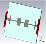
The characteristics of the designed microstrip low-pass filter are given in Table 1. The circuit model for the microstrip low-pass filter is shown in Figure 1.

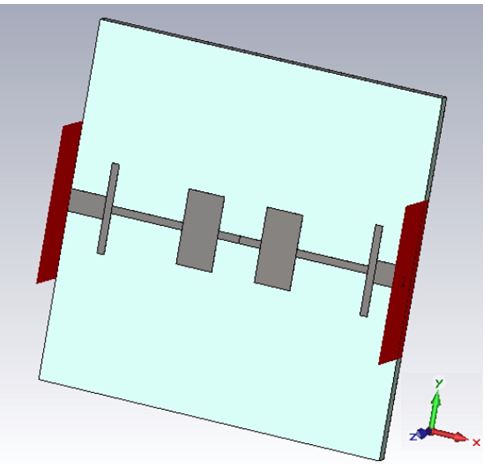
Fig. 1. 3D circuit model for eight-layer symmetrical microstrip low-pass filter.

B. Modeling parameter detection

The low training cost to be obtained is achieved by determining the optimum connection weights of the network. The selection of the input data set is very important for the determination of these optimum connection weights. The input parameter (electrical length g $_{i}$ ) ranges to be used in order to train the network in the widest range with the most optimum results were selected in the range of 0.5 $-$ 2.6 from the results of an optimization study [23]. These values are in the widest range band and include the ranges used in other studies [23, 24]. As it is known, optimization processes are long and costly processes. For this reason, the modeling process with the appropriate data set in many subjects provides a convenient and low-cost opportunity in terms of time. In addition, data reduction is frequently used in such applications in a way that does not change the result obtained from the analysis. For this, a sampling technique called LHS was chosen and modified according to the objectives of the present study. Data reduction method was used by taking the widest range selected for each layer as a reference.

LHS is a popular stratified sampling technique first proposed by MacKay [25] and further developed by Iman and Conover [26]. It is a sampling method of random designs that try to be evenly distributed in the design space. With the LHS, one must first decide how many sample points to use and remember in which row and column the sample point is taken for each sample point. This configuration is similar to having N rooks on a chessboard without threatening each other [25, 26]. Here, the electrical lengths (g $_{i}$ ) of the eight-layer symmetrical filter are selected in the ranges given in Table 2. Equal step spacing was chosen as 0.05 so that there are 100 frequency samples in total.

Table 2: Data set

Parameter	Range	Sampling	Number of
Parameter	Range	Method	Samples
g $_{i}$	0.50 $-$ 2.6	LHS	225
Frequency (GHz)	0.05 $-$ 5.0	Linear	100
Train sample	$-$	$-$	(225/2) $\times$
Train sample	$-$	$-$	100
Validation	$-$	$-$	(225/2) $\times$
sample	$-$	$-$	100

III. MLP MODEL FOR MICROSTRIP LOW-PASS FILTER ANALYSIS

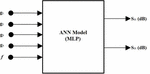
MLP-type multi-layer ANNs consist of input, hidden, and output layers. The structure of the network allows multi-element input/output modeling [27]. The MLP model used in this design is designed for different parameters consisting of two, three, and four hidden layers and consisting of 5, 10, 15, and 20 neurons. Similar structures have given successful results for a different study before [16]. Neurons input/output layers have different weight coefficients. In the training phase, modeling continues until the resulting training error rate is minimized [27]. For this purpose, a combination of two different activation functions was used between the layers. As the activation function in the hidden layer, logsis is preferred in the last neuron and tansig is preferred for the other layers. The output obtained as a result of each iteration is compared with the target, and depending on the error given, the network training is continued with the weight renewal process or the training process is terminated. The total input to the neurons of each layer is obtained by weighting the neuron outputs in a lower layer. The training success of the network can be achieved by adjusting these different weight coefficients correctly. This adjustment is compared with the output values in the previous step and corrected in the next step. Of course, besides these, it is very important to create the accurate network model. While creating the network model, there are a total of five input parameters, including four electrical length (g $_{i}$ ) parameters and frequency, which are different because the filter has a symmetrical structure. The black box model of the proposed network structure is given in Figure 2.

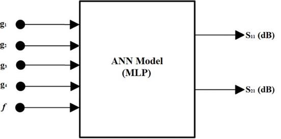
Fig. 2. ANN model for training S $_{11}$ and S $_{21}$ (dB) parameters of microstrip low-pass filter.

A. Activation functions

In this study, the activation functions used between layers for MLP type ANNs are, respectively, tangent-sigmoid (tansig) and logarithmic-sigmoid (logsig).

Tansig: The neuron input $-$ output expression for this activation function is given in eqn (1) and the change of the function is given in Figure 3 (a). The dynamic range of change of the function is the range [ $-$ 1 1], and the function neuron shows a non-linear change in this range depending on the total input. This function is also called the hyperbolic-tangent function in the literature

a = 2 / (1 + e^{(- 2 n)}) - 1 .

(1)

Logsig: The input $-$ output expression of this activation function, which is also called the sigmoid function, and the change of the function according to the input are given in eqn (2) and Figure 3 (b), respectively. The dynamic range of the function is the range [0 1], and the function exhibits a non-linear change in this range

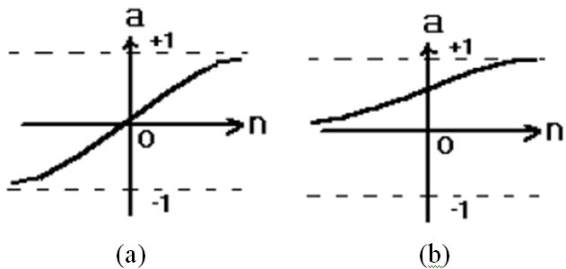
Fig. 3. (a) Tangent-sigmoid function input $-$ output curve. (b) Logarithmic-sigmoid function input $-$ output curve.

a = 1 / (1 + e^{- n}) .

(2)

B. Training algorithms

There are various training algorithms used to train the selected network. Here, we will explain three different neural network algorithms that we used while creating the algorithm. These algorithms are trainbr (Bayesian regularization), trainlm (quasi-Newton), and trainrp (gradient descent) [28].

Trainbr: Bayesian regression algorithm is a network training function in which the weight values and bias corresponding to the Levenberg $-$ Marquardt optimization are updated. It reduces the combination of weights and squared errors to determine the appropriate combination that will help develop an important generalized quality network, and this whole process is known as Bayesian editing. Also, this function has some disadvantages such as using Jacobian for calculations; where performance is assumed to be the mean or sum of squared errors. Therefore, all structures/networks trained with the trainbr function should use either the mean of squared errors or the sum of squared errors [29].

Trainlm: Quasi-Newton algorithm provides preferred and fast optimization over conjugate gradient algorithms. It is based on the Hessian matrix (second derivatives) of the performance function with respect to the current values of the weights and deviations. It provides faster convergence than conjugate gradient methods. Because of its complexity, it takes a lot of time to find the Hessian matrix for FFNN. It is also known as the secant method and does not need any quadratic calculations. The Hessian matrix is updated very closely in all iterations of the algorithms. Trainlm is an iterative approach where the performance function will always be reduced in all iterations of the algorithm. Therefore, it becomes the fastest training algorithm for networks with a modest size. It also detects the minimum of a multi-variate function, which is the sum of the squares of non-linear real-valued functions. Besides its advantages, it has some limitations such as storage problem and computational overhead [30].

Trainrp: Gradient descent algorithms are popularized training algorithms that perform the basic gradient descent algorithm that changes the weights and biases toward the negative gradient of the performance function. The elasticity back propagation (trainrp) training algorithm cancels out the results of the weights of the partial derivatives [31]. In this algorithm, the derivative sign is used to decide whether to update the weights, and the size of the derivative does not affect the weight update. The weight change amount is learned with an independent update value. If the first derivative of the performance function by weight is of equal magnitude for two consecutive iterations [32], the update value is raised by a factor for each weight and deviation, and the same weight changes from the previous iteration. If the derivative is zero, the update will stay the same, and if the weights are flickering, they will be reduced.

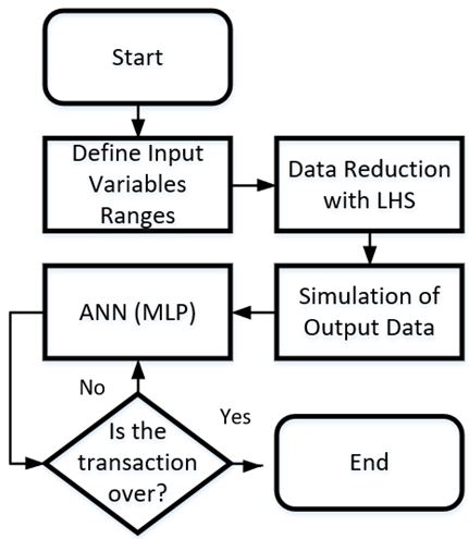
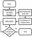
Fig. 4. Flow chart of modeling process of LHS- and MLP-based low-pass filter.

IV. CASE STUDY

In the study part, a modeling study will be made for the ISM band application of the MLP-based eight-layer non-uniform microstrip filter. The proposed eight-layer microstrip filter is formed with a symmetrical structure. In this symmetric model, there are eight microstrip transmission lines, four of which are different. Therefore, based on the ANN model in Figure 2, the microstrip filter consists of five variables in total, including the frequency that will directly affect the output parameters S $_{11}$ and S $_{21}$ (dB). Training and validation data sets (Table 1) to construct the proposed MLP-based microstrip filter model are obtained using the EM simulation tool for the selected substrate FR4 (h = 1.6 mm; $ε$ $_{r}$ = 4.4). For the intervals given in Table 2, the data set is created using the LHS method. Here, the number of training and test data reduced for training is 225 $\times$ 100 in total. This input data is sized with the aid of a microstrip line calculator to obtain the results of S $_{11}$ and S $_{22}$ (dB) at each sample frequency. The resulting data sets are randomly divided into half as training and test data. This training and test data are processed with predetermined MLP algorithms and architectures (a total of 21 different types). All these applied processes are presented in Figure 4 as a flow chart. Since MLP algorithms are based on randomly initiated conditions and processes, the microstrip filter design is evaluated for 10 different runs to determine the best, worst, and mean performance of each MLP model to determine the most stable architecture for the optimization problem.

The following are the commonly used error metrics used for performance evaluation of MLP models: mean absolute error (MAE) (eqn (3)); relative mean absolute error (RMAE) (eqn (4))

MAE = \frac{1}{N} \sum_{i = 1}^{N} | T_{i} - P_{i} |

(3)

RMAE = \frac{1}{N} \sum_{i = 1}^{N} \frac{| T_{i} - P_{i} |}{| T_{i} |}

(4)

where N is the total number of samples, T is the target value, and P stands for predicted value.

Table 3: Performance comparison of ANN models based on MAE

Algorithm	Architecture	Max.	Min.	Mean
trainbr	5 10	2.09	1.96	2.01
	10 15	1.58	1.32	1.47
	15 20	1.40	0.98	1.17
	5 10 15	0.93	0.81	0.88
	5 15 20	1.00	0.76	0.90
	10 15 20	0.91	0.55	0.74
	5 10 15 20	0.66	0.49	0.62
trainlm	5 10	2.21	2.09	2.16
	10 15	1.76	1.20	1.47
	15 20	1.32	1.09	1.12
	5 10 15	4.17	0.66	2.60
	5 15 20	1.17	0.76	0.97
	10 15 20	0.79	0.67	0.69
	5 10 15 20	1.06	0.63	0.80
trainrp	5 10	2.92	2.76	2.83
	10 15	2.46	2.34	2.38
	15 20	2.41	2.18	2.28
	5 10 15	2.66	2.43	2.55
	5 15 20	2.75	2.35	2.41
	10 15 20	2.12	1.81	1.99
	5 10 15 20	2.37	2.26	2.34

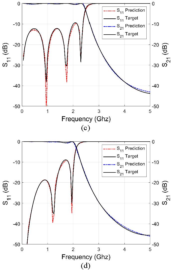
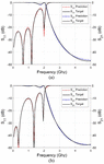
Fig. 5. Result of EM simulation and MLP-based modeling with the trainbr algorithm, ${$ 5-10-15-20 $}$ with hidden layers for eight-layer low-pass filter as S $_{11}$ and S $_{21}$ parameters: (a) g $_{1}$ $_{- 7}$ = 1.48; g $_{2}$ $_{- 6}$ = 1.97; g $_{3}$ $_{- 5}$ = 2.18; g $_{4}$ = 1.7; g $_{8}$ = 1. (b) g $_{1}$ $_{- 7}$ = 1.71; g $_{2}$ $_{- 6}$ = 2.04; g $_{3}$ $_{- 5}$ = 1.91; g $_{4}$ = 2.28; g $_{8}$ = 1. (c) g $_{1}$ $_{- 7}$ = 1.68; g $_{2}$ $_{- 6}$ = 1.19; g $_{3}$ $_{- 5}$ = 2.45; g $_{4}$ = 1.23; g $_{8}$ = 1. (d) g $_{1}$ $_{- 7}$ = 1.17; g $_{2}$ $_{- 6}$ = 2.06; g $_{3}$ $_{- 5}$ = 1.9; g $_{4}$ = 2.11; g $_{8}$ = 1.

The performance measures obtained in 10 different runs for the 21 different ANN models identified are given in Table 3. Here, the MAE value is used in the overall comparison of the models during the validation process. The error value decreases with the increase in the number of hidden layers in the architecture used. However, among the algorithms used, trainbr (Bayesian regression) has the best results. As a result, among the results in Table 3, ${$ 5-10-15-20 $}$ trained with the trainbr method and the model trained with four hidden layers and hidden neurons has the best performance criteria in terms of both minimum error and narrow max $-$ min range. The results selected from ${$ 5-10-15-20 $}$ trained with Bayesian regression method and the model trained with four hidden layers and hidden neurons. In Figure 5 (a) $-$ (d), S $_{11}$ and S $_{21}$ (dB) values were obtained by ANN. The estimated prediction is shown with the MATLAB program as target data obtained with the 3D EM simulation tool CST. As can be seen in the graphics, a high success has been achieved.

Finally, performance comparisons were made with other ANN models, especially XGBoosting-based ensemble learning, which has been popular recently in the best result surrogate model designs found with the proposed model. The parameters and results used in XGBoosting, radial basis function (RBF), and general regression neural network (GRNN) models are given numerically in Table 4. As can be seen from the results, the proposed model has the lowest error result.

Table 4: Performance comparison with other ANN models based on MEA

Model	Hyperparameter	Test Error
MLP	Hidden layer = 4neuron = [5 10 15 20]	0.49
RBF	Spread = 0.215	1.42
GRNN	Spread = 0.181	1.67
Ensemble	Method: bag, Number of cycles: 488, Min. leaf size: 1 Max. number of splits: 3344	1.8 $\pm$ 0.2

V. CONCLUSION

Here, the modeling of the fast, practical, and reliable S $_{11}$ and S $_{21}$ (dB) parameters of the non-uniform microstrip filter is discussed using MLP for certain design features. The total number of samples was kept to a minimum by using the LHS method in the selection of training and test data. The proposed model is also low-cost in terms of total number of samples and computation [4, 19]. Performance comparisons were made for different algorithms and architectures using the created data sets. Thus, the most successful algorithm and architecture were determined. Algorithms and architectures used in the proposed MLP model have been chosen from those that have proven successful for a different design problem [16]. As a result of the study, it was seen that the ANN modeling used and 225 samples were used as accurately as an EM simulator for other electrical lengths (g $_{i}$ ) parameters in a wide range selected. In addition, the proposed model is not only limited to a non-uniform microstrip filter but can also be successfully applied to other microwave circuit design problems by changing the design optimization aim.

REFERENCES

[1] J-S. G. Hong and M. J. Lancaster, Microstrip Filters for RF/Microwave Applications, 1st Edition. John Wiley & Sons Inc., 2001.

[2] R. E. Zich, M. Mussetta, F. Grimaccia, A. Gandelli, H. M. Linh, G. Agoletti, M. Bertarini, L. Combi, P. F. Scaramuzzino, and A. Serboli, “Comparison of different optimization techniques in microstrip filter design,” IEEE Asia-Pacific International Microwave Symposium on Electromagnetic Compatibility (APEMC), pp. 549-552, May 2012.

[3] Y. Jiang and X. Nong, “A radar filtering model for aerial surveillance base on kalman filter and neural network,” IEEE 11th International Conference on Software Engineering and Service Science (ICSESS), pp. 57-60, Oct. 2020.

[4] T. Mahouti, N. Kuşkonmaz, and T. Yıldırım, “Modelling of non-planar microstrip lines via artificial neural networks,” Innovations in Intelligent Systems and Applications Conference (ASYU), Nov. 2019.

[5] N. Türker and F. Güneş, “An artificial neural model of the microstrip lines,” Proceedings of the IEEE 12th Signal Processing and Communications Applications Conference, pp. 657-660, Apr. 2004.

[6] L. Sorokosz and W. Zieniutycz, “Electromagnetic modeling of microstrip elements aided with artificial neural network,” Baltic URSI Symposium (URSI), pp. 85-88, Nov. 2020.

[7] P. T. Selvan and S. Raghavan, “A CAD neural analysis for conductor backed asymmetric CPW with one lateral ground plane,” International Conference on Computer, Communication and Electrical Technology (ICCCET), pp. 266-270, May 2011.

[8] G. L. Creech, B. J. Paul, C. D. Lesniak, T. J. Jenkins, and M. C. Calcatera, “Artificial neural networks for fast and accurate EM-CAD of microwave circuits,” IEEE Trans. Microwave Theory Tech., vol. 45, no. 5, pp. 794-802, May 1997.

[9] A. H. Zaabab, Q. J. Zhang, and M. S. Nakhla, “A neural network modeling approach to circuit optimization and statistical design,” IEEE Trans Microwave Theory Tech., vol. 43, no. 6, pp. 1349-1358, Jun. 1995.

[10] M. C. E. Yagoub, “Active device modeling methodologies for RF/microwave system-level CAD,” 25th Annual Review of Progress in Applied Computational Electromagnetics, pp. 155-160, Mar. 2009.

[11] F. Güneş, P. Mahouti, S. Demirel, M. A. Belen, and A. Uluslu, “Cost-effective GRNN-based modeling of microwave transistors with a reduced number of measurements,” International Journal of Numerical Modelling: Electronic Networks, Devices and Fields, vol. 30, no. 3-4, May 2017.

[12] F. Güneş, S. Demirel, and S. Nesil, “A novel design approach to XBand Minkowski Reflectarray antennas using the full-wave EM simulation-based complete neural model with a hybrid GA-NM algorithm,” Radioengineering, vol. 23, no. 1, pp. 144-153, Apr. 2014.

[13] P. Mahouti, F. Gunes, A. Caliskan, and M. A. Belen, “A novel design of non-uniform Reflectarrays with symbolic regression and its realization using 3-D printer,” Applied Computational Electromagnetics Society Journal, vol. 34, no. 2, pp. 280-285, Feb. 2019.

[14] D. Krishna, J. Narayana, and D. Reddy, “ANN models for microstrip line synthesis and analysis,” World Academy of Science, Engineering and Technology, International Science Index 22, International Journal of Electrical, Computer, Energetic, Electronic and Communication Engineering, vol. 2, no. 10, pp. 2343-2347, Nov. 2008.

[15] P. Mahouti, F. Güneş, M. A. Belen, and S. Demirel, “Symbolic regression for derivation of an accurate analytical formulation using “Big Data” an application example,” Applied Computational Electromagnetics Society Journal, vol. 32, no 5, pp. 372-380, May 2017.

[16] P. Mahouti, “Design optimization of a pattern reconfigurable microstrip antenna using differential evolution and 3D EM simulation-based neural network model,” International Journal of RF and Microwave Computer-Aided Engineering, vol. 29, no. 8, Aug. 2019.

[17] G. S. Tomar, V. S. Kushwah and S. Saxena, “Design of microstrip filters using neural network,” Second International Conference on Communication Software and Networks, pp. 568-572, Feb. 2010.

[18] V. S. Kushwah, G. S. Tomar and S. S. Bhadauria, “Designing stepped impedance microstrip low-pass filters using artificial neural network at 1.8 GHz,” International Conference on Communication Systems and Network Technologies, pp. 11-16, Apr. 2013.

[19] T. Mahouti, T. Y $ı$ ld $ı$ r $ı$ m, and N. Kuşkonmaz, “Artificial intelligence–based design optimization of nonuniform microstrip line band pass filter,” International Journal of Numerical Modelling, vol. 34, no. 6, Apr. 2021.

[20] D. M. Pozar, Microwave Engineering, 2nd Edition, John Wiley, 2000.

[21] https://www.emtalk.com/mscalc.php

[22] J-S. G. Hong and M. J. Lancaster, Microstrip Filters for RF/ Microwave Applications. John Wiley & Sons Inc, 2001.

[23] A. Uluslu, “Microstrip low pass filter analysis and design,” Research & Reviews in Engineering, Gece Publishing, vol. 1, pp. 35-52, May 2021.

[24] H. Bohra and A. Ghosh, “Design and analysis of microstrip low pass and bandstop filters,” International Journal of Recent Technology and Engineering (IJRTE), vol. 8, no. 3, pp. 6944-6951, Sep. 2019.

[25] M. MaKa, R. Beckman, and W. Conover, “A comparison of three methods for selecting values of input variables in the analysis of output from computer code,” Technimeterics, vol. 21, no. 1, pp. 239-245, May 1979.

[26] R. Iman and W. Conover, “Small sample sensitivity analysis techniques for computers models, with an application to risk assessment,” Communications in Statistics - Theory and Methods, vol. 9, no. 17, pp. 1749-1842, Jan. 1980.

[27] Z. Şen, Yapay Sinir Ağlar $ı$ İlkeleri, Su Vakfı Yayınları, İstanbul, 2004.

[28] S. Ali and K. A. Smith, “On learning algorithm selection for classification,” Applied Soft Computing, vol. 6, no. 2, pp. 119-138, Jan. 2006.

[29] http://in.mathworks.com/help/nnet/ref/trainbr.html

[30] D. Pham and S. Sagiroglu, “Training multilayered perceptrons for pattern recognition: a comparative study of four training algorithms,” International Journal of Machine Tools and Manufacture, vol. 41, no. 3, pp. 419-430, Feb. 2001.

[31] A. D. Anastasiadis, G. D. Magoulas, and M. N. Vrahatis, “New globally convergent training scheme based on the resilient propagation algorithm,” Neurocomputing, vol. 64, pp. 253-270, Mar. 2005.

[32] http://www-rohan.sdsu.edu/doc/matlab/toolbox/nnet/backpr57.html

BIOGRAPHIES

Ahmet Uluslu received the Ph.D. degree from the Electronics and Communication Engineering Department, Istanbul Y $ı$ ld $ı$ z Technical University, Istanbul, Turkey, in 2020. He received the master’s degree from the Department of Electromagnetic Fields and Microwave Techniques, Istanbul Y $ı$ ld $ı$ z Technical University. He is currently working as a Lecturer with Istanbul University - Cerrahpaşa Electronics and Automation Department. His current research areas are microwave circuits, especially optimization techniques of microwave circuits, antenna design, and antenna optimization and modeling.