Interaction Magnetic Force of Cuboidal Permanent Magnet and Soft Magnetic Bar Using Hybrid Boundary Element Method

Ana N. Vučković¹, Mirjana T. Perić¹, Saša S. Ilić¹, Nebojša B. Raičević¹, and Dušan M. Vučković²

¹Department of Theoretical Electrical Engineering, University of Niš, Faculty of Electronic Engineering,

18000 Niš, Serbia

{ana.vuckovic, mirjana.peric, sasa.ilic, nebojsa.raicevic}@elfak.ni.ac.rs

²Department of Computer Science, University of Niš, Faculty of Electronic Engineering, 18000 Niš, Serbia

dusan.vuckovic@elfak.ni.ac.rs

Submitted On: June 16, 2021; Accepted On: October 30, 2021

Abstract

The hybrid boundary element method for solving a three-dimensional magnetostatic problem is presented in this paper for the first time. The interaction force between the cuboidal permanent magnet and the bar, made of soft magnetic material, is calculated. Results of the presented approach are confirmed using COMSOL Multiphysics as well as with the results of the image theorem that is applicable when the dimensions of the bar are large enough; so it could be considered an infinite soft magnetic plane.

Index Terms: Hybrid boundary element method (HBEM), magnetization charges, magnetic force, cuboidal permanent magnet.

I. INTRODUCTION

In order to precisely calculate performance parameters of different electronic devices, various mathematical methods can be applied. Efficiency of the most common ones in the analysis of the problems involving electromagnetic fields of very thin electrodes [1] is debatable. Some of these applications were analyzed in the cable terminations having a thin deflector [2], strip lines with perfect conducting plates [3], or floating stripes used for electrostatic field modeling [4].

Since there is a constant need for size reduction and optimization of electrical devices and gadgets, the development of new mathematical approaches for their performance’s calculation is a necessity. The hybrid boundary element method (HBEM) developed at the Department of Theoretical Electrical Engineering was initially made for solving electromagnetic field distribution in the vicinity of cable joints and terminations [5, 6], but it finds its application in solving numerous electromagnetic problems. As a combination of the boundary element method (BEM) [7], the equivalent electrodes method (EEM) [8], and the point-matching method (PMM), until now, it was applied for permanent magnets (PMs) configuration modeling [9, 10], characteristic parameters of transmission lines calculation [11, 12, 13], and for the grounding system analyses [14]. Also, a line inductance of two-wire in the vicinity of magnetic material composites was successfully calculated using this approach [15]. All the structures that are analyzed using HBEM are either planar or axially symmetrical, but the method can be used for solving 3D electromagnetic problems too. The advantage of the method is that equivalent electrodes, equivalent currents, or magnetic sources, depending on the problem that is being solved, are located on the body surface, or boundary surface between two different materials, while in the case of the charge simulation method (CSM), sources are placed within the volume.

The application of HBEM for 3D magnetostatic problems is presented here for the first time. It will be applied to a PM configuration modeling because, due to the low production cost, PMs have become a primary choice in many instances. The absence of a power supply unit also goes in favor of PMs. Perfect examples are magnetic couplings, bearings, different assemblies, sensors, or actuators. Cuboidal, cylindrical, and ring magnets are the most common shapes of PMs and many scientists around the world are calculating the field, force, and torque of different configurations that contain them [16, 17, 18, 19, 20, 21]. Since Akoun presented his study of cuboidal PMs [22], many papers were published that were dealing with the force and torque between cuboidal magnets using Ampere’s current [23, 24] or magnetic charges approach [16, 19, 20, 25, 26, 27]. Also, the calculation of the interaction between a cuboidal magnet and current carrying conductor [28] or a cuboidal magnet and infinite magnetic plate are the topics of interest [29]. The HBEM was applied for calculating the force between ring and cylindrical PM and the object of the finite dimension made of soft magnetic material [9, 10].

This method is used in the paper for the force calculation between cuboidal magnet and the bar made of soft magnetic material. The advantages of this approach are its simplicity and low computation time. The results presented could prove important in the modeling and manufacturing process of different devices that incorporate PMs.

II. METHODOLOGY

The basic idea of the HBEM is that either the conductor surface or the boundary surfaces between two dielectric layers or even boundary surface between two different magnetic materials should be divided first into number of small segments. For the electrostatic problems, equivalent electrodes or electric charges should be placed right in the center of each segment. Influence of the magnetic materials of different magnetic permittivity can be replaced by equivalent currents that are located on the boundary surface of the magnetic layers. Using the boundary condition for tangential components of magnetization vector on boundary surface of two magnetic materials, $M_{2\mathrm{t}}-M_{1\mathrm{t}}=J_{\mathrm{s}},$ a system of linear equations can be formed with microscopic Ampere’s currents, $J_{\mathrm{s}}$, as the unknown values [5].

The system of magnetic sources placed along the boundary surface also substitutes the influence of two different magnetic materials. In that case, the system of linear equations is formed using the boundary condition for the normal component of magnetization vector on the boundary surface, $M_{2\mathrm{n}}-M_{1\mathrm{n}}={\eta }_{\mathrm{m}}$ [9, 10].

The geometry of the sources depends on the problem that is being solved. In case of axial symmetry, the magnetic sources are toroidal [9, 10], for the planar problems, they are line charges [13, 14], and for 3D problems, magnetic sources are spherically shaped.

A. Model definition

Using HBEM, the system of cuboidal PM and the bar made of soft magnetic material is modeled (Figure 1).

The PM magnetized in the axial direction is modeled using the fictitious magnetic charges approach. Since the boundary conditions for the surface and volume charge density have to be satisfied [30]

$${\eta }_{\mathrm{m}}=\widehat{n}\cdot \mathit{\text{M}},$$

(1)

$${\rho }_{\mathrm{m}}=-\nabla \cdot \mathit{\text{M}}=0,$$

(2)

it is obvious that the magnetic charges exist on the bottom and the top faces of the magnet, with the surface density ${\eta }_{\mathrm{m1}}=\widehat{n}\cdot \mathit{\text{M}}=M$ for the top face, and ${\eta }_{\mathrm{m2}}=\widehat{n}\cdot \mathit{\text{M}}=-M$, for the bottom one [25]. The volume charge density is equal to zero.

On the other hand, since the bar is made of soft magnetic material of magnetic permeability $\mu ={\mu }_0{\mu }_{\mathrm{r2}}$, its influence can be replaced with a system of small airborne spherical magnetic sources. Boundaries between the soft magnetic bar and the air (all faces of the magnetic bar) are divided into a large number of square-shaped segments. Each magnetic source is located in the center of a segment. The discretization model of the system is presented in the Figure 2.

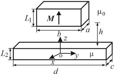
Fig. 1. Cuboidal magnet placed above soft magnetic bar.

Fig. 2. Discretization model for the considered system.

B. HBEM application

The magnetic scalar potential of magnetic sources system

$${\phi }_{\mathrm{m}}=\sum _{n=1}^N{Q}_{n}G(\mathit{\text{r}},{\mathit{\text{r}}}_{\mathit{\text{n}}})$$

(3)

can be calculated starting from the Green’s function of an isolated point magnetic charge

$$G(\mathit{\text{r}},{\mathit{\text{r}}}_{\mathit{\text{n}}})=\frac{1}{4\pi \left|\mathit{\text{r}}-{\mathit{\text{r}}}_{\mathit{\text{n}}}\right|},$$

(4)

where r is the field point radius vector and ${\mathit{\text{r}}}_{\mathit{\text{n}}}$ is the radius vector of the spherical magnetic source center.

After the discretization (Figure 2), the magnetic scalar potential of the considered system becomes

$${\phi }_{\mathrm{m}}=\sum _{k=1}^{N_a{N}_b}(\frac{Q_{\mathrm{k}}^{\mathrm{m}}}{4\pi \sqrt{{\left(x-x_k\right)}^2+{\left(y-y_k\right)}^2+{\left(z-z_{k1}\right)}^2}}$$

$$-\frac{Q_{\mathrm{k}}^{\mathrm{m}}}{4\pi \sqrt{{\left(x-x_k\right)}^2+{\left(y-y_k\right)}^2+{\left(z-z_{k2}\right)}^2}})+$$

$$+\sum _{i=1}^{N_{\mathrm{tot}}}\frac{Q_i}{4\pi }\frac{1}{\sqrt{{\left(x-x_i\right)}^2+{\left(y-y_i\right)}^2+{\left(z-z_i\right)}^2}}.$$

(5)

The first sum in eqn (5) is the magnetic scalar potential of the PM. The magnetic charges of the PM segments are $Q_{\mathrm{k}}^{\mathrm{m}}=M\frac{ab}{N_{\mathrm{a}}{N}_{\mathrm{b}}}$.

The positions of the top face elements are $(x_k,y_k,$ $z_{k1}=h+L_1+L_2\mathrm{/}2)$ and for the bottom ones are $(x_k,y_k,$ $z_{k2}=h+L_2\mathrm{/}2)$.

$N_a\cdot N_b$ is the total number of the surface charges on the PM face. $N_a$ and $N_b$ are the number of the segments along the edges $a$ and $b$, calculated from the initial number of segments (magnetic point charges) N. They depend on the PM dimensions, $N_a=\sqrt{aN\mathrm{/}b}$ and $N_b=N\mathrm{/}\sqrt{aN\mathrm{/}b}$.

The second sum in eqn (5) represents the magnetic scalar potential of the bar made of soft magnetic material. Each face of the bar is discretized into square segments with corresponding spherical magnetic sources, $Q_i$, placed in the center of each segment.

The radii of the spherical sources placed along the faces of the bar are

$a_{\mathrm{e}z}=\sqrt{\frac{\mathrm{\Delta }x\mathrm{\Delta }y}{2\pi }}$, for the bottom and the top faces,

$a_{\mathrm{e}x}=\sqrt{\frac{\mathrm{\Delta }z\mathrm{\Delta }y}{2\pi }}$, for the front and back faces,

$a_{\mathrm{e}y}=\sqrt{\frac{\mathrm{\Delta }x\mathrm{\Delta }z}{2\pi }}$, for the right and left faces,

where $\mathrm{\Delta }x=\frac{N_d}{d},\mathrm{\Delta }y=\frac{N_c}{c},\mathrm{\Delta }z=\frac{N_L}{L_2}$.

$N_d,N_c,\mathrm{and}{N}_L$ are the number of the segments along the edges $d,c,\mathrm{and}{L}_2$ that are calculated starting from the initial number of the elements, $N_{\mathrm{s}}$. So, the total number of segments (or unknown magnetic sources $Q_i$) is $N_{\mathrm{tot}}=2N_c{N}_d+2N_c{N}_L+2N_d{N}_L$.

Magnetic field strength vector can be expressed as

$$\mathit{\text{H}}=-\mathrm{grad}\left({\phi }_{\mathrm{m}}\right).$$

(6)

The relation that the normal component of the magnetic field vector and surface charges must complete is

$${\widehat{n}}_k\cdot H_k=-\frac{{\mu }_{\mathrm{r2}}}{{\mu }_{\mathrm{r1}}-{\mu }_{\mathrm{r2}}}{\eta }_{\mathrm{m}i},$$

(7)

$${\eta }_{\mathrm{m}i}=\frac{Q_i}{S_i},i=1,2,\mathrm{\dots },N_{\mathrm{tot}},k=1,\mathrm{\dots },6,$$

where ${\widehat{n}}_k$ is the outgoing unit normal vector and $S_i$ is the surface of the ith segment.

The system of the linear equations is formed after the point matching method is applied for the normal component of the magnetic field. The solution of the linear equations system gives the values of unknown boundary sources of the bar $Q_i$. After the magnetic sources are calculated, the magnetic scalar potential of the bar becomes

$${\phi }_{\mathrm{mb}}=\frac{1}{4\pi }\sum _{i=1}^{N_{\mathrm{tot}}}\frac{Q_i}{\sqrt{{\left(x-x_i\right)}^2+{\left(y-y_i\right)}^2+{\left(z-z_i\right)}^2}}.$$

(8)

The magnetic field vector can be determined by the expression (6), and magnetic flux density vector in the vicinity of the bar is

$${\mathit{\text{B}}}^{\mathit{\text{ext}}}={\mu }_0{\mathit{\text{H}}}^{\mathit{\text{ext}}}.$$

(9)

Finally, when magnetic flux density vector generated by the bar is determined, the interaction force can be calculated using the superposition of the force obtained between all sources of the bar and all magnetic charges of the PM:

$$\mathit{\text{F}}=\sum _{k=1}^{N_a{N}_b}{Q}_k^m{\mathit{\text{B}}}^{\mathit{\text{ext}}}.$$

(10)

Substituting eqn (9) in eqn (10), the force is calculated, and its components are

	$F_x={\displaystyle \frac{{\mu }_0}{4\pi }}{\displaystyle \frac{Mab}{N_a{N}_b}}\times$	(11)
	${\displaystyle \sum _{k=1}^{N_a{N}_b}}{\displaystyle \sum _{i=1}^{N_{\mathrm{tot}}}}{Q}_i({\displaystyle \frac{x_k-x_i}{{\left({\left(x_k-x_i\right)}^2+{\left(y_k-y_i\right)}^2+{\left(z_{k1}-z_i\right)}^2\right)}^{\frac{3}{2}}}}-$
	$-{\displaystyle \frac{x_k-x_i}{{\left({\left(x_k-x_i\right)}^2+{\left(y_k-y_i\right)}^2+{\left(z_{k2}-z_i\right)}^2\right)}^{\frac{3}{2}}}}),$

	$F_y={\displaystyle \frac{{\mu }_0}{4\pi }}{\displaystyle \frac{Mab}{N_a{N}_b}}\times$
	${\displaystyle \sum _{k=1}^{N_a{N}_b}}{\displaystyle \sum _{i=1}^{N_{\mathrm{tot}}}}{Q}_i({\displaystyle \frac{y_k-y_i}{{\left({\left(x_k-x_i\right)}^2+{\left(y_k-y_i\right)}^2+{\left(z_{k1}-z_i\right)}^2\right)}^{\frac{3}{2}}}}-$

$$-\frac{y_k-y_i}{{\left({\left(x_k-x_i\right)}^2+{\left(y_k-y_i\right)}^2+{\left(z_{k2}-z_i\right)}^2\right)}^{\frac{3}{2}}}),$$

(12)

	$F_z={\displaystyle \frac{{\mu }_0}{4\pi }}{\displaystyle \frac{Mab}{N_a{N}_b}}\times$
	${\displaystyle \sum _{k=1}^{N_a{N}_b}}{\displaystyle \sum _{i=1}^{N_{\mathrm{tot}}}}{Q}_i({\displaystyle \frac{z_{k1}-z_i}{{\left({\left(x_k-x_i\right)}^2+{\left(y_k-y_i\right)}^2+{\left(z_{k1}-z_i\right)}^2\right)}^{\frac{3}{2}}}}-$

$$-\frac{z_{k2}-z_i}{{\left({\left(x_k-x_i\right)}^2+{\left(y_k-y_i\right)}^2+{\left(z_{k2}-z_i\right)}^2\right)}^{\frac{3}{2}}}).$$

(13)

The x and y components of the force are equal to zero; so the calculated z component represents the interaction force.

III. NUMERICAL RESULTS

The expression for the interaction force, developed using HBEM, is easily handled in the Wolfram Mathematica environment and enables parametric studies of the force. The results are presented graphically for the different configuration parameters.

Convergence of the results is tested, and the results are compared with the finite-element method (FEM) (COMSOL Multiphysics) computations in order to determine the optimal number of magnetic sources. For the system parameters: $a\mathrm{/}{L}_1=b\mathrm{/}{L}_1=2.0,$$h\mathrm{/}{L}_1=1.0$,$c\mathrm{/}{L}_1=d\mathrm{/}{L}_1=4.0,$ $L_2\mathrm{/}{L}_1=2.0,$ $M=750kA\mathrm{/}m,$ ${\mu }_r=100$, $N=3000$, the attraction force is calculated for various numbers of bar segments, $N_{\mathrm{s}},$ as it is presented in Figure 3. The same configuration is modeled in COMSOL Multiphysics and the obtained intensity of the force is 3.4617 N. In the case when the initial number of segments is $N_{\mathrm{s}}=7000$, the relative deviation between FEM and HBEM result is 0.58%. It is confirmed that the HBEM results are compliant with the value obtained with FEM. In the further calculations, the number of PM segments is limited to $N=3000$ and the initial number of the bar segments is $N_{\mathrm{s}}=7000$.

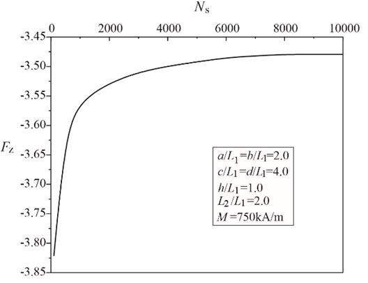
Fig. 3. Convergence results.

The results of the presented approach are also compared with the ones obtained using the method of images [23, 25] for the case where the dimensions of the bar, $c\mathrm{/}{L}_1,d\mathrm{/}{L}_1$ are large enough; so it could be considered an infinite soft magnetic plane. Figure 4 presents comparative results of three different methods. The normalized magnetic force, $F_z{}^{nor}=$$F_z\mathrm{/}{\mu }_0{M}^2{L}_1^2$, versus relative permeability of the bar, for various axial displacements of the magnet is shown. Configuration parameters are: $a\mathrm{/}{L}_1=b\mathrm{/}{L}_1=3.0,$ $c\mathrm{/}{L}_1=d\mathrm{/}{L}_1=18.0.$ Results shown in Figure 4 also prove the accuracy of the method. HBEM results coincide with the image theorem results, with relative deviation lower than 0.6%. FEM results, on the other hand, have a relative deviation below 1.5%.

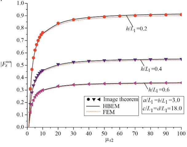
Fig. 4. Interaction force versus relative magnetic permeability ${\mu }_{\mathrm{r2}}$.

Table 1 presents the computational time in case where HBEM, image theorem, and FEM were applied. The computational time is the lowest in case of the image theorem, but a disadvantage of this approach is that it is not applicable when the bar is of finite dimension.

Table 1: Computational time

	HBEM	Image Theorem	FEM
CPU time [s]	39.4	28.6	129

The comparative results of HBEM and FEM are presented in Figures 5–9 with the satisfactory alignment.

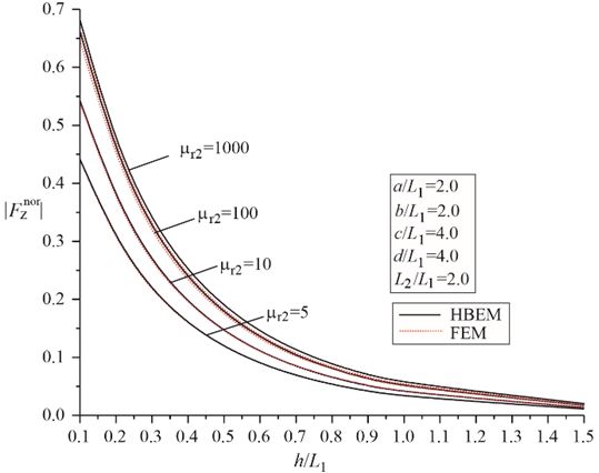
Fig. 5. Interaction force versus $h\mathrm{/}{L}_1$ for variable magnetic permeability ${\mu }_{\mathrm{r2}}$.

Fig. 6. Interaction force versus $h\mathrm{/}{L}_1$ for different values of PM dimensions.

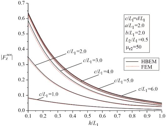
Fig. 7. Interaction force versus $h\mathrm{/}{L}_1$ for different values of bar’s dimensions.

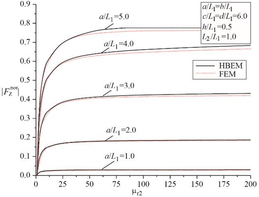
Fig. 8. Interaction force versus relative magnetic permeability of the bar for variable PM dimensions.

Normalized axial force between PM and soft magnetic bar versus normalized axial displacement of PM, $h\mathrm{/}{L}_1$, for variable relative permeability of the bar, ${\mu }_{\mathrm{r2}}$, is presented in Figure 5. The analysis is performed for $a\mathrm{/}{L}_1=b\mathrm{/}{L}_1=2.0,$ $c\mathrm{/}{L}_1=d\mathrm{/}{L}_1=4.0,L_2\mathrm{/}{L}_1=2.$

Figures 6 and 7 present interaction force distribution versus the distance $h\mathrm{/}{L}_1$ for different values of PM dimensions and for various bar’s dimensions, respectively. The system parameters in the first case are: $c\mathrm{/}{L}_1=d\mathrm{/}{L}_1=3.0,$ $L_2\mathrm{/}{L}_1=1,$${\mu }_{\mathrm{r2}}=100$, while in the second example: ${\mu }_{\mathrm{r2}}=50$, $a\mathrm{/}{L}_1=b\mathrm{/}{L}_1=2.0,$ $L_2\mathrm{/}{L}_1=0.5$.

Force distribution versus relative permeability of the bar is presented in Figures 8 and 9 with the configuration parameters: $c\mathrm{/}{L}_1=d\mathrm{/}{L}_1=6.0,$ $L_2\mathrm{/}{L}_1=1.0,$$h\mathrm{/}{L}_1=0.5$ and $a\mathrm{/}{L}_1=3.0,$ $b/L_1=1.0,$ $c\mathrm{/}{L}_1=5.0,$ $h\mathrm{/}{L}_1=0.2$,$h\mathrm{/}{L}_1=0.5$, respectively.

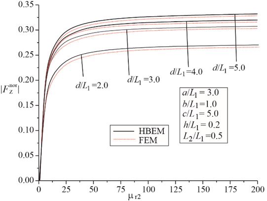
Fig. 9. Interaction force versus relative magnetic permeability ${\mu }_{\mathrm{r2}}$ for variable bar’s dimensions.

IV. CONCLUSION

The HBEM is applied for the calculation of the interaction force between cuboidal PM and the bar made of soft magnetic material. The three-dimensional electromagnetic problem is solved for the first time using this approach. The accuracy of the method is confirmed using COMSOL Multiphysics software and the image theorem. The solution for the magnetostatic problem is derived here, and, similarly, using analogous procedure, the wide variety of multilayer 3D electromagnetic problems can be solved. The advantage of this method is its simplicity. Since the discretization of the surface is applied, it is also very time efficient. As expected, the number of segments grows with the increase in dimensions of the bar. For the examples presented in the paper, it is not greater than $N_{\mathrm{s}}=7000$. Calculation done using Intel i7 processor and 32 GB of RAM took around 15 minutes of run time for a distribution curve. Parametric studies and design of the devices that incorporate PMs could be improved using the obtained expression of the force.

ACKNOWLEDGMENT

This work has been supported by the Ministry of Education, Science and Technological Development of the Republic of Serbia.

REFERENCES

[1] C. A. Brebbia, J. C. F. Telles, and L. C. Wrobel, Boundary Element Techniques. Theory and Applications in Engineering, Springer, Berlin, 1984.

[2] N. B. Raičević, “Conformal mapping and equivalent electrodes method application of electric field determination at cable accessories,” Discrete and Computational Mathematics, Nova Publishers, New York, USA, chapter 14, pp. 205-214, 2008.

[3] N. B. Raičević and S. S. Ilić, “Equivalent electrode method application on anisotropic micro strip lines calculations,” Int. Conf. on Electromagnetics in Advanced Applications ICEAA 07, Torino, Italy, paper 122 (CD), Sep. 2007.

[4] N. B. Raičević, “One method for multilayer dielectric system determination,” 8th Int. Conf. on Applied Electromagnetics PES 2007, Niš, Serbia, Sep. 2007.

[5] N. B. Raičević, S. R. Aleksić, and S. S. Ilić, “A hybrid boundary element method for multi-layer electrostatic and magnetostatic problems,” Journal of Electromagnetics, no. 30, pp. 507-524, 2010.

[6] N. B. Raičević, S. S. Ilić, and S. R. Aleksić, “Application of new hybrid boundary element method on the cable terminations,” 14th International IGTE Symposium, Graz, Austria, pp. 56-61, Sep. 2010.

[7] D. Li and L. Di. Rizenzo, “Boundary element computation of line parameters of on-chip interconnects on lossy silicon substrate,” Applied Computational Electromagnetics Society (ACES) Journal, vol. 26, no. 9, pp. 716-722, Sep. 2011.

[8] D. M. Veličković, “Equivalent electrodes method,” Scientific Review, no. 21-22, pp. 207-248, 1996.

[9] A. N. Vučković, D. M. Vuckovic, M. T. Perić, and N. B. Raičević, “Influence of the magnetization vector misalignment on the magnetic force of permanent ring magnet and soft magnetic cylinder,” International Journal of Applied Electromagnetics and Mechanics, vol. 65, no. 3, pp. 417-430, Mar. 2021.

[10] A. N. Vučković, N. B. Raičević, and M. T. Perić, “Radially magnetized ring permanent magnet modelling in the vicinity of soft magnetic cylinder,” Safety Engineering, vol. 8, no. 1. pp. 33-37, Jun. 2018.

[11] S. Ilić, M. Perić, S. Aleksić, and N. Raičević, “Hybrid boundary element method and quasi-TEM analysis of 2D transmission lines – generalization,” Electromagnetics, vol. 33, no. 4, pp. 292-310, Apr. 2013.

[12] M. T. Perić, S. S. Ilić, S. R. Aleksić, and N. B. Raičević, “Application of hybrid boundary element method to 2D microstrip lines analysis,” International Journal of Applied Electromagnetics and Mechanics, vol. 42, no. 2, pp. 179-190, 2013.

[13] M. T. Perić, S. S. Ilić, A. N. Vučković, and N. B. Raičević, “Improving the efficiency of hybrid boundary element method for electrostatic problems solving,” Applied Computational Electromagnetics Society (ACES) Journal, vol. 35, no. 8, pp. 872-877, Aug. 2020.

[14] S. S. Ilić, N. B. Raičević, and S. R. Aleksić, “Application of new hybrid boundary element method on grounding systems,” 14th International IGTE Symposium, Graz, Austria, pp. 160-165, Sep. 2010.

[15] S. Ilić, D. B. Jovanović, A. N. Vučković, and M T. Perić, “External inductance per unit length calculation of two wire line in vicinity of linear magnetic material,” 14th Int. Conf. on Applied Electromagnetics PES 2019, Niš, Serbia, Sep. 2019.

[16] H. Allag, J.P. Yonnet, H. Bouchekara, M. Latreche, and C. Rubeck, “Coulombian model for 3D analytical calculation of the torque exerted on cuboidal permanent magnets with arbitrary oriented polarizations,” Applied Computational Electromagnetics Society (ACES) Journal, vol. 30, no. 4, pp. 351-356, Apr. 2015.

[17] J. Ren, L.Yang, and J. Ren, “Study on spatial magnetic field intensity distribution of rectangular permanent magnets based on Matlab,” Applied Computational Electromagnetics Society Conference, vol. 46, no. 1, pp. 255-269, 2014.

[18] A. N. Vučković, N. B. Raičević, S. S. Ilić, and S. R. Aleksić, “Interaction magnetic force calculation of radial passive magnetic bearing using magnetization charges and discretization technique,” International Journal of Applied Electromagnetics and Mechanics, vol. 43, no. 4, pp. 311-323, 2013.

[19] W. S. Robertson, B. S. Cazzolato, and A. C. Zander, “A simplified force equation for coaxial cylindrical magnets and thin coils,” IEEE Transactions on Magnetics, vol. 47, pp. 2045-2049, Aug. 2011.

[20] R. Ravaud, G. Lemarquand, and V. Lemarquand, “Force and stiffness of passive magnetic bearings using permanent magnets. Part 1: Axial magnetization,” IEEE Transactions on Magnetics, vol. 45, pp. 2996-3002, Jul. 2009.

[21] M. Lahdo, T. Strohla, and S. Kovalev, “Magnetic propulsion force calculation of a 2-DoF large stroke actuator for high-precision magnetic levitation system,” Applied Computational Electromagnetics Society (ACES) Journal, vol. 32, no. 8, pp. 663-669, Aug. 2017.

[22] G. Akoun and J. P. Yonnet, “3D analytical calculation of the forces exerted between two cuboidal magnets,” IEEE Transactions on Magnetics, vol. 20, pp. 1962-1964, Sep. 1984.

[23] Ana N. Vučković, Saša S. Ilić, and Slavoljub R. Aleksić, “Interaction magnetic force calculation of ring permanent magnets using Ampere’s microscopic surface currents and discretization technique,” Electromagnetics, vol. 32, no. 2, pp. 117-134, Jan. 2012.

[24] M. Braneshi, O. Zavalani, and A. Pijetri, “The use of calculating function for the evaluation of axial force between two coaxial disk coils,” Third International PhD Seminar on Computational Electromagnetics and Technical Application, Banja Luka, Bosnia and Hertzegovina, pp. 21–30, Aug. 2006.

[25] A. N. Vučković, S. R. Aleksić, and S. S. Ilić, “Calculation of the attraction and levitation forces using magnetization charges,” 10th Int. Conf. on Applied Electromagnetics PES 2011, CD Proceedings, Niš, Serbia, pp. 33-55, Sep. 2011.

[26] J. L. G. Janssen, J. J. H. Paulides, and E. A. Lomonova, “3-D analytical calculation of the torque between perpendicular magnetized magnets in magnetic suspension,” IEEE Trans. on Magnetics, vol. 47, no. 10, pp. 4286-4289, Oct. 2011.

[27] H. Allag and J. P. Yonnet, “3-D Analytical calculation of the torque and force exerted between two cuboidal magnets,” IEEE Trans. on Magnetics, vol. 45, no. 10, pp. 3969-3972, Oct. 2009.

[28] M. Aissaoui, H. Allag, and J. P. Yonnet, “Mutual inductance and interaction calculation between conductor or coil of rectangular cross section andparallelepiped permanent magnet,” IEEE Trans. on Magnetics, vol. 50, no. 11, Nov. 2014.

[29] M. Beleggia, D. Vokoun, and M. D. Graef, “Forces between a permanent magnet and a soft magnetic plate,” IEEE Magnetics Letters, vol. 3, 2012.

[30] E. P. Furlani, Permanent Magnet and Electromechanical Devices: Materials, Analysis and Applications, Academic Press, London, 6th edition, 2001.

ACES JOURNAL, Vol. 36, No. 11, 1492–1498.
doi: 10.13052/2021.ACES.J.361114
© 2021 River Publishers

Abstract

I. INTRODUCTION

II. METHODOLOGY

A. Model definition

B. HBEM application

III. NUMERICAL RESULTS

IV. CONCLUSION

ACKNOWLEDGMENT

REFERENCES