Spatial Processing Using High-Fidelity Models of Dual-Polarization Antenna Elements

John N. Spitzmiller and Sanyi Y. Choi

Integration and Production Program Directorate
Parsons, Huntsville, AL 35806, USA
john.spitzmiller@parsons.com, sanyi.choi@parsons.com

Submitted On: August 27, 2021; Accepted On: October 18, 2021

Abstract

This paper generalizes a recent improvement to a traditional spatial-processing algorithm to optimally use body-mounted arrays of dual-polarization radio-frequency antenna elements rather than single-polarization antenna elements. The paper’s generalized algorithm exploits high-fidelity far-field gain and polarization data, generated most practically by a computational electromagnetic solver (CES), to characterize the antenna array’s individual dual-polarization elements. Using this characterization and that of the desired and undesired communication nodes’ antennas, the generalized algorithm determines the array’s optimal weights. The subsequent application of a CES to a practical scenario, in which an optimally weighted array of dual-polarization antenna elements is mounted on a representative body, demonstrates the generalized algorithm’s exceptional spatial-processing performance.

Keywords: antenna arrays, beamforming, nullsteering, polarization matching, spatial filters, spatialprocessing.

I. INTRODUCTION

This paper generalizes a recent improvement [1] to a traditional algorithm for spatial processing (beamforming in the direction of a single desired communication node and nullsteering in the directions of potentially multiple undesired communication nodes). The recent algorithmic improvement optimally used an array of potentially diverse single-polarization radio-frequency (RF) antenna elements arbitrarily arranged on a body of arbitrary shape and material composition. This paper generalizes that improved algorithm to optimally use arrays of dual-polarization antenna elements. A dual-polarization antenna element has two ports, each of which corresponds to one of two nominally orthogonal polarizations in the direction of the element’s maximum gain. For example, the two polarizations could be orthogonally linear (say, vertical and horizontal) or orthogonally circular (i.e., right-hand circular (RHC) and left-hand circular (LHC)). This paper assumes the antenna array functions exclusively in a receive mode. However, under the assumed principle of reciprocity [2], this paper’s generalized spatial-processing algorithm applies equally to a transmitting antenna array.

Previous research in spatial processing with arrays of dual-polarization elements [3, 4, 5, 6, 7, 8, 9, 10] has recognized this problem’s extraordinary complexity in even relatively simple practical scenarios. For example, the electrical effects caused by surface waves on the body, mutual coupling between array elements, and spatial variations in element gain and polarization patterns are practically impossible to characterize without a full-wave computational electromagnetic solver (CES) solution or sophisticated measurements [3]. In response researchers have generally made three simplifying assumptions to facilitate their analyses and simulations. Firstly, most researchers assume the absence of any tangible body [3, 4, 5, 6] on which the antenna array is mounted. This assumption precludes the study of surface-wave effects that are crucial to scenarios in which the body is physically between an emitter and the receiving antenna [11] or antenna array [1]. Although some researchers [7, 8, 9, 10] assume a planar or cylindrical physical layout of the antenna elements, they still account for no explicit body in their analyses. Secondly, most researchers explicitly assume negligible mutual coupling between the array’s elements [3, 4, 5, 6, 7, 9, 10]. Thirdly, most researchers assume the array’s dual-polarization elements are ideal crossed-dipole (or electrically equivalent) elements which have perfectly orthogonally linear transmission and reception characteristics [4, 5, 6, 7, 9, 10].

Since these effects are typically small, much meaningful research can be performed while ignoring them. However, the accurate characterization of a spatial-processing algorithm’s performance in practical scenarios requires exceptional fidelity in all three typically simplified areas. For example, to achieve extremely deep nulls in a receive array’s gain pattern, a spatial-processing algorithm must weight the element output signals so that their sum is nearly exactly zero. By maximally exploiting the high-fidelity data produced by a CES, this paper’s generalized algorithm accounts for the typically small yet non-negligible electrical effects of the presence of the body, mutual coupling between array elements, and element gain and polarization deviations from ideal behavior.

All traditional receive-mode spatial-processing algorithms [12, 13, 14] require knowledge of the array elements’ locations in the receive array’s coordinate system, the thermal-noise power-spectral density (PSD) at every array output port, the desired and undesired far-field emitters’ apparent angular directions in the array’s coordinate system, and all undesired emitters’ spatial power densities at the array’s location. This paper’s generalized algorithm requires additional information. Specifically, the generalized algorithm requires quantitative knowledge (or, at least, estimates) of the desired and undesired emitters’ antenna gains and polarization characteristics in the direction of the receive array. The algorithm also requires high-fidelity quantitative knowledge of the transmitted far-field vector electric field in the directions of all scenario emitters produced by each port of each array element, accounting for the structure of the corresponding element, the electromagnetic interactions with the other elements (i.e., mutual-coupling effects), and the electromagnetic interactions with the body. Only a CES or high-fidelity testing can practically provide such detailed data. Proper processing of this additional information produces the parameters needed to populate the recently developed, high-fidelity RF antenna models (both transmit and receive modes) [15, 16].

Using the populated antenna models, the generalized algorithm calculates a set of complex weights (effecting amplitude scalings and phase shifts) to apply to the output signals of the array elements’ ports. The summation of these weighted signals optimizes some appropriate figure of merit (e.g., the signal-to-interference ratio (SIR) when the array operates in an RF-interference (RFI) environment). These signal modifications effectively produce an antenna pattern having high effective gain in the direction of the desired emitter and low effective gains in the directions of the undesired emitters. Note that effective gain is the total gain less the polarization-mismatch loss, which is ideally very low for the desired emitter and very high for all undesiredemitters.

Section II reviews this problem’s technical background. Section III generalizes the spatial-processing technique of [1] assuming dual-polarization antenna elements. Section IV presents high-fidelity digital-simulation results for an array of realistic dual-polarization antenna elements mounted on a representative body. Section V concludes the paper with a summary of key results and several suggestions for future work.

II. TECHNICAL BACKGROUND

This section reviews the technical background needed for the development of Section III’s generalized algorithm. Subsection A provides the general scenario’s physical description, including the locations of the receive-antenna elements, the single desired emitter, and the potentially multiple undesired emitters. Subsection B mathematically specifies the desired and undesired emitters’ transmitted signals. Subsections C, D, and E respectively characterize the receive-antenna array’s elements, the desired emitter’s antenna, and the undesired emitters’ antennas. Subsection F derives the electric fields incident on the receive-antenna elements. Subsection G develops the array elements’ output signals. Subsection H describes the receiver/spatial-processor model fed by the receive-antenna array’s elements. Section I presents the problem statement.

A. Physical description of scenario

The diagram of Figure 1 notionally depicts the scenario of interest. A receive-antenna array mounted on a body of potentially complex shape and material composition attempts to receive an RF signal from a desired far-field emitter. Multiple spatially diverse undesired far-field RF emitters interfere with the desired signal’s reception. Note that the body may be physically between one or more of the receive array’s elements and one or more of the scenario’s emitters.

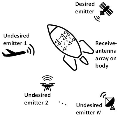
Figure 1: Notional depiction of scenario.

Figure 2 shows the basic scenario geometry in which an array of M dual-polarization antenna elements arranged on a body receives signals from a single desired far-field emitter and N undesired far-field emitters. The Cartesian coordinate system shown in Figure 2 has its origin at O, some convenient point near the physical center of the antenna array on the body. Figure 2 also shows a spherical coordinate system using the traditional quantities of the distance r (r $\ge$ 0) and the two orthogonal angles $\theta (0\le \theta \le \pi )$ and $\varphi (0\le \varphi <2\pi )$ to specify an arbitrary point of interest.

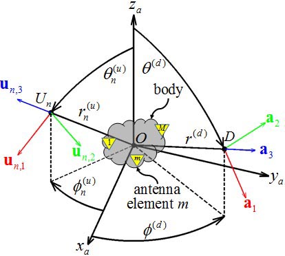
Figure 2: Basic scenario geometry.

The single desired emitter’s antenna’s phase center, located at D, has spherical coordinates $(r^{(d)},{\theta }^{(d)},{\varphi }^{(d)})$ and Cartesian coordinates

$\left[\begin{array}{c}\hfill x^{(d)}\hfill \\ \hfill y^{(d)}\hfill \\ \hfill z^{(d)}\hfill \end{array}\right]=\left[\begin{array}{c}\hfill r^{(d)}{s}_{{\theta }^{(d)}}{c}_{{\varphi }^{(d)}}\hfill \\ \hfill r^{(d)}{s}_{{\theta }^{(d)}}{s}_{{\varphi }^{(d)}}\hfill \\ \hfill r^{(d)}{c}_{{\theta }^{(d)}}\hfill \end{array}\right],$

(1)

where we use the shorthand notation

$\left[\begin{array}{cc}\hfill c_{\rho }\hfill & \hfill s_{\rho }\hfill \end{array}\right]=\left[\begin{array}{cc}\hfill \cos (\rho )\hfill & \hfill \sin (\rho )\hfill \end{array}\right]\forall \rho \in ℝ.$

(2)

The nth undesired emitter’s antenna’s phase center, located at U${}_n$, has spherical coordinates $(r_n^{(u)},{\theta }_n^{(u)},{\varphi }_n^{(u)})$ and Cartesian coordinates

$\left[\begin{array}{c}\hfill x_n^{(u)}\hfill \\ \hfill y_n^{(u)}\hfill \\ \hfill z_n^{(u)}\hfill \end{array}\right]=\left[\begin{array}{c}\hfill r_n^{(u)}{s}_{{\theta }_n^{(u)}}{c}_{{\varphi }_n^{(u)}}\hfill \\ \hfill r_n^{(u)}{s}_{{\theta }_n^{(u)}}{s}_{{\varphi }_n^{(u)}}\hfill \\ \hfill r_n^{(u)}{c}_{{\theta }_n^{(u)}}\hfill \end{array}\right],n\in \{1,\mathrm{\cdots },N\}.$

(3)

The phase center of the $m$th element’s $p$th port has Cartesian coordinates (x${}_{m\mathrm{,}p}$${}^{\mathrm{(}}$${}^a$${}^{\mathrm{)}}$, y${}_{m\mathrm{,}p}$${}^{\mathrm{(}}$${}^a$${}^{\mathrm{)}}$, z${}_{m\mathrm{,}p}$${}^{\mathrm{(}}$${}^a$${}^{\mathrm{)}}$).

As shown in Figure 2, we define three orthogonal unit vectors associated with the antenna array and the desired emitter. Firstly, unit vector

${𝐚}_3={\left[\begin{array}{ccc}\hfill s_{{\theta }^{(d)}}{c}_{{\varphi }^{(d)}}\hfill & \hfill s_{{\theta }^{(d)}}{s}_{{\varphi }^{(d)}}\hfill & \hfill c_{{\theta }^{(d)}}\hfill \end{array}\right]}^T,$

(4)

with T denoting simple (unconjugated) transposition, points along the ray from O to D (i.e., in the direction of increasing distance from O at D). Secondly, unit vector

${𝐚}_1={\left[\begin{array}{ccc}\hfill c_{{\varphi }^{(d)}}{c}_{{\theta }^{(d)}}\hfill & \hfill s_{{\varphi }^{(d)}}{c}_{{\theta }^{(d)}}\hfill & \hfill -s_{{\theta }^{(d)}}\hfill \end{array}\right]}^T,$

(5)

points in the direction of the antenna array’s increasing $\theta$ at D. Thirdly, unit vector

${𝐚}_2={\left[\begin{array}{ccc}\hfill -s_{{\varphi }^{(d)}}\hfill & \hfill c_{{\varphi }^{(d)}}\hfill & \hfill 0\hfill \end{array}\right]}^T,$

(6)

points in the direction of the antenna array’s increasing $\varphi$ at D. Unit vectors a${}_{\mathrm{1}}$ and a${}_{\mathrm{2}}$ are parallel to all planes normal to the line passing through O and D. Thus, for any point on this line, the plane defined by these unit vectors contains the polarization ellipse of a plane electromagnetic (EM) wave propagating between D and O.

As shown in Figure 2, we define three orthogonal unit vectors associated with the antenna array and the nth undesired emitter. Firstly, unit vector

${𝐮}_{n,3}={\left[\begin{array}{ccc}\hfill s_{{\theta }_n^{(u)}}{c}_{{\varphi }_n^{(u)}}\hfill & \hfill s_{{\theta }_n^{(u)}}{s}_{{\varphi }_n^{(u)}}\hfill & \hfill c_{{\theta }_n^{(u)}}\hfill \end{array}\right]}^T,$

(7)

points along the ray from O to U${}_n$ (i.e., in the direction of increasing distance from O at U${}_n$). Secondly, unit vector

${𝐮}_{n,1}={\left[\begin{array}{ccc}\hfill c_{{\varphi }_n^{(u)}}{c}_{{\theta }_n^{(u)}}\hfill & \hfill s_{{\varphi }_n^{(u)}}{c}_{{\theta }_n^{(u)}}\hfill & \hfill -s_{{\theta }_n^{(u)}}\hfill \end{array}\right]}^T,$

(8)

points in the direction of the antenna array’s increasing $\theta$ at U${}_n$. Thirdly, unit vector

${𝐮}_{n,2}={\left[\begin{array}{ccc}\hfill -s_{{\varphi }_n^{(u)}}\hfill & \hfill c_{{\varphi }_n^{(u)}}\hfill & \hfill 0\hfill \end{array}\right]}^T,$

(9)

points in the direction of the antenna array’s increasing $\varphi$ at U${}_n$. Unit vectors u${}_n$${}_{\mathrm{,}\mathrm{1}}$ and u${}_n$${}_{\mathrm{,}\mathrm{2}}$ are parallel to all planes normal to the line passing through O and U${}_n$. Thus, for any point on this line, the plane defined by these unit vectors contains the polarization ellipse of a plane EM wave propagating between U${}_n$ and O.

As shown in Figure 3, unit vector

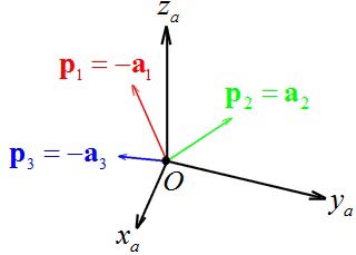
Figure 3: Unit vectors associated with the desired emitter.

${𝐩}_3=-{𝐚}_3,$

(10)

points along the ray from D to O. We define the orientation of the desired emitter’s local spherical coordinate system, having origin at D, to satisfy two requirements. Firstly, unit vector

${𝐩}_1=-{𝐚}_1,$

(11)

points in the direction of the desired emitter’s increasing $\theta$ at O. Secondly, unit vector

${𝐩}_2={𝐚}_2,$

(12)

points in the direction of the desired emitter’s increasing $\varphi$ at O. Unit vectors p${}_{\mathrm{1}}$ and p${}_{\mathrm{2}}$ define planes normal to the line passing through O and D. Thus, for any point on this line, the plane defined by these unit vectors contains the polarization ellipse of a plane EM wave propagating between D and O.

As shown in Figure 4, unit vector

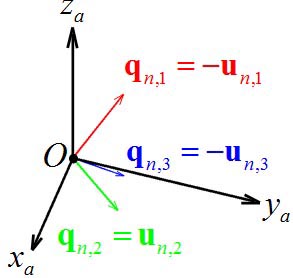
Figure 4: Unit vectors associated with the nth undesired emitter.

${𝐪}_{n,3}=-{𝐮}_{n,3},$

(13)

points along the ray from U${}_n$ to O. We define the orientation of the nth undesired emitter’s local spherical coordinate system, having origin at U${}_n$, to satisfy two requirements. Firstly, unit vector

${𝐪}_{n,1}=-{𝐮}_{n,1},$

(14)

points in the direction of the nth undesired emitter’s increasing $\theta$ at O. Secondly, unit vector

${𝐪}_{n,2}={𝐮}_{n,2},$

(15)

points in the direction of the $n$th undesired emitter’s increasing $\varphi$ at O. Unit vectors q${}_n$${}_{\mathrm{,}\mathrm{1}}$ and q${}_n$${}_{\mathrm{,}\mathrm{2}}$ define planes normal to the line containing O and U${}_n$. Thus, for any point on this line, the plane defined by these unit vectors contains the polarization ellipse of a plane EM wave propagating between U${}_n$ and O.

B. Mathematical description of transmitted signals

The desired emitter’s transmitter sends to its antenna the deterministic narrowband signal

$x^{(d)}(t)=A^{(d)}(t)\cos \left[2\pi f_{RF}t+{\gamma }^{(d)}(t)\right],$

(16)

where A${}^{\mathrm{(}}$${}^d$${}^{\mathrm{)}}$(t) and $\gamma$${}^{(}$${}^d$${}^{)}$(t) are the narrowband signal’s slowly varying amplitude modulation and phase modulation, respectively, f${}_{R\mathit{}F}$ is the center RF in hertz, and t is time in seconds. Assuming the desired emitter’s antenna has unit impedance, the desired emitter’s time-averaged power is

$P^{(d)}={\left[A^{(d)}\right]}^2\mathrm{/}2,$

(17)

if we also assume A${}^{\mathrm{(}}$${}^d$${}^{\mathrm{)}}$(t) is a constant A${}^{\mathrm{(}}$${}^d$${}^{\mathrm{)}}$.

The nth undesired emitter’s transmitter sends to its antenna the zero-mean, wide-sense stationary (WSS) random narrowband signal

$x_n^{(u)}(t)=x_{I,n}^{(u)}(t)\cos (2\pi f_{RF}t)-x_{Q,n}^{(u)}(t)\sin (2\pi f_{RF}t),$

(18)

where x${}_I$${}_{\mathrm{,}n}$${}^{\mathrm{(}}$${}^u$${}^{\mathrm{)}}$(t) and x${}_Q$${}_{\mathrm{,}n}$${}^{\mathrm{(}}$${}^u$${}^{\mathrm{)}}$(t) are, respectively, the inphase (I) and quadrature (Q) components of x${}_n$${}^{\mathrm{(}}$${}^u$${}^{\mathrm{)}}$(t). We assume the N undesired emitters’ signals are mutually uncorrelated.

The nth undesired emitter’s signal has double-sided PSD

$S_n^{(u)}(f)=\frac{N_n^{(u)}}{2}\left[\mathrm{\Pi }\left(\frac{f-f_{RF}}{B_n^{(u)}}\right)+\mathrm{\Pi }\left(\frac{f+f_{RF}}{B_n^{(u)}}\right)\right],$

(19)

where N${}_n$${}^{\mathrm{(}}$${}^u$${}^{\mathrm{)}}$/2 is the PSD’s level in W/Hz, B${}_n$${}^{\mathrm{(}}$${}^u$${}^{\mathrm{)}}$ is the bandwidth in Hz, and

$\mathrm{\Pi }(x)=\{\begin{array}{cc}\hfill 1,\hfill & \hfill |x|\le 1/2\hfill \\ \hfill 0,\hfill & \hfill \mathrm{otherwise}\hfill \end{array},$

(20)

is the unit pulse function. The nth undesired emitter’s I and Q components are independent, zero-mean, WSS random lowpass processes with double-sided PSD

$S_{I,n}^{{}^{(u)}}(f)=S_{Q,n}^{{}^{(u)}}(f)=N_n^{(u)}\mathrm{\Pi }\left(f/B_n^{(u)}\right).$

(21)

C. Electrical description of antenna array

We assume complete quantitative knowledge of the practically planar vector electric field

$\begin{array}{c}{𝐄}_{m,p}^{(a)}(t,r^{(a)},\theta ,\varphi ,f_{RF})=\hfill \\ {𝐯}_1(\theta ,\varphi )E_{m,p,1}^{(a)}(r^{(a)},\theta ,\varphi ,f_{RF})\hfill \\ \times \cos [2\pi f_{RF}t+{\gamma }_{m,p,1}^{(a)}(r^{(a)},\theta ,\varphi ,f_{RF})]\hfill \\ +{𝐯}_2(\theta ,\varphi )E_{m,p,2}^{(a)}(r^{(a)},\theta ,\varphi ,f_{RF})\hfill \\ \times \cos [2\pi f_{RF}t+{\gamma }_{m,p,2}^{(a)}(r^{(a)},\theta ,\varphi ,f_{RF})]\hfill \end{array},$

(22)

produced at known far-field slant range r${}^{\mathrm{(}}$${}^a$${}^{\mathrm{)}}$ from O for every combination of $\theta$ and $\varphi$ corresponding to a scenario emitter when monochromatic source signal

$s_s(t)=A_s\cos (2\pi f_{RF}t+{\gamma }_s),$

(23)

exclusively stimulates port p of array element m with all elements present on the body. In (22) direction-dependent unit vector v${}_i$, i$\mathrm{\in }$$\mathrm{\{}$1,2$\}$, can represent a${}_i$ or u${}_n$${}_{\mathrm{,}}$${}_i$ as appropriate. Equation (22) is the electric field produced at a point with spherical coordinates (r${}^{\mathrm{(}}$${}^a$${}^{\mathrm{)}}$, $\theta$, $\varphi$) when element m is transmitting due to the stimulation by (23) of only its pth port while all other elements are physically present but electrically inactive. A CES is the most practical source of such high-fidelity data, but sophisticated testing might be capable of generating these data. Figure 5 shows the high-fidelity antenna model [15] corresponding to the pth port of the antenna array’s mth element. The model has two sets of direction-dependent parameters. The first set comprises an apparent internal attenuation K${}_m$${}_{\mathrm{,}}$${}_p$${}_{\mathrm{,}\mathrm{1}}$${}^{\mathrm{(}}$${}^a$${}^{\mathrm{)}}$($\theta$,$\varphi$) and an apparent internal delay $\tau$${}_m$${}_{,}$${}_p$${}_{,1}$${}^{(}$${}^a$${}^{)}$($\theta$,$\varphi$) associated with an antenna perfectly linearly polarized along ${𝐯}_1$. The second set comprises an apparent internal attenuation K${}_m$${}_{\mathrm{,}}$${}_p$${}_{\mathrm{,}\mathrm{2}}$${}^{\mathrm{(}}$${}^a$${}^{\mathrm{)}}$($\theta$,$\varphi$) and an apparent internal delay $\tau$${}_m$${}_{,}$${}_p$${}_{,2}$${}^{(}$${}^a$${}^{)}$($\theta$,$\varphi$) associated with a collocated antenna perfectly linearly polarized along v${}_{\mathrm{2}}$.

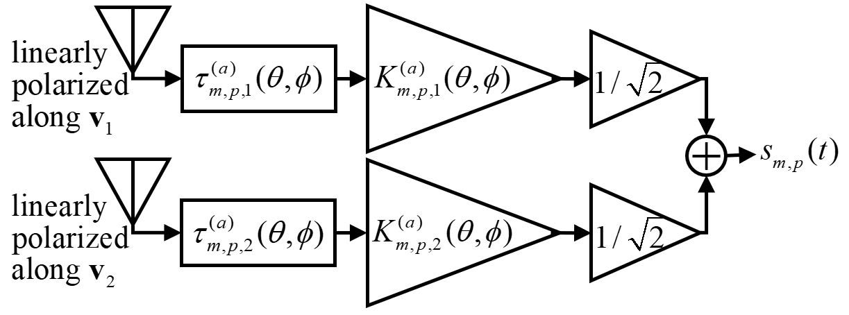
Figure 5: Model for the $p$th port of the antenna array’s mth element.

The model’s apparent internal attenuations are

$\begin{array}{c}{K}_{m,p,i}^{(a)}(r^{(a)},\theta ,\varphi ,f_{RF})=\hfill \\ \frac{\sqrt{2}{E}_{m,p,i}^{(a)}(r^{(a)},\theta ,\varphi ,f_{RF})}{A_s}{K}^{(a)},i\in \{1,2\},\hfill \end{array}$

(24)

where [16]

$K^{(a)}=\lambda r^{(a)}/Z_0.$

(25)

In (25) the EM wave’s wavelength is

$\lambda =c/f_{RF},$

(26)

where c is the speed of light (exactly 299,792,458 m/s in free space, the assumed propagation medium). Also, in (25) Z${}_{\mathrm{0}}$ = 4$\pi$$\times$10${}^{-7}$c $\approx$ 376.7303 $\mathrm{\Omega }$ is the intrinsic impedance of free space.

The model’s apparent internal time delays are

$\begin{array}{c}{\tau }_{m,p,i}^{(a)}(\theta ,\varphi ,f_{RF})\approx \frac{{\gamma }_s-{\gamma }_{m,p,i}^{(a)}(r^{(a)},\theta ,\varphi ,f_{RF})}{2\pi f_{RF}}\hfill \\ -r^{(a)}/c+k_{m,p,i}^{(a)}/f_{RF}\hfill \\ +\left[s_{\theta }{c}_{\varphi }{x}_{m,p}^{(a)}+s_{\theta }{s}_{\varphi }{y}_{m,p}^{(a)}+c_{\theta }{z}_{m,p}^{(a)}\right]\mathrm{/}c,i\in \{1,2\},\hfill \end{array}$

(27)

where k${}_{m\mathrm{,}p}$${}_{\mathrm{,}}$${}_i$${}^{\mathrm{(}}$${}^a$${}^{\mathrm{)}}$ is any integer satisfying

$\begin{array}{c}{\gamma }_{m,p,i}^{(a)}(r^{(a)},\theta ,\varphi ,f_{RF})={\gamma }_s+2\pi k_{m,p,i}^{(a)}\hfill \\ -2\pi f_{RF}\left[r^{(a)}+s_{\theta }{c}_{\varphi }{x}_{m,p}^{(a)}+s_{\theta }{s}_{\varphi }{y}_{m,p}^{(a)}+c_{\theta }{z}_{m,p}^{(a)}\right]\mathrm{/}c\hfill \\ -2\pi f_{RF}{\tau }_{m,p,i}^{(a)}(r^{(a)},\theta ,\varphi ,f_{RF}).\hfill \end{array}$

(28)

We intuitively choose each k${}_{m\mathrm{,}p}$${}_{\mathrm{,}}$${}_i$${}^{\mathrm{(}}$${}^a$${}^{\mathrm{)}}$ to make the corresponding $\tau$${}_{m,p}$${}_{,}$${}_i$${}^{(}$${}^a$${}^{)}$ positive but minimal. Note that (24) and (27) account for the presence of the body and the other antenna elements. In other words, for each of the array’s $2M$ ports, this technique produces apparent internal attenuations and delays which generally differ—often significantly—from the apparent internal attenuations and delays obtained in the absence of the other antenna elements and the body.

D. Electrical description of desired emitter’s antenna

We assume the desired emitter’s transmit antenna has a known total gain of G${}^{\mathrm{(}}$${}^d$${}^{\mathrm{)}}$ in the direction of O. We further assume the desired emitter’s transmit antenna has a known polarization characterized by axial ratio R${}^{\mathrm{(}}$${}^d$${}^{\mathrm{)}}$, tilt angle $\alpha$${}^{(}$${}^d$${}^{)}$, and rotation sense s${}^{\mathrm{(}}$${}^d$${}^{\mathrm{)}}$ in the direction of O. The phase difference $\delta$${}^{(}$${}^d$${}^{)}$ between the untilted spatially orthogonal electric field components appearing in the far field is [16]

${\delta }^{(d)}=\{\begin{array}{cc}\hfill -\pi /2,\hfill & \hfill s^{(d)}=R\hfill \\ \hfill \pi /2,\hfill & \hfill s^{(d)}=L\hfill \end{array}.$

(29)

Given these characteristics, we model the desired emitter’s transmit antenna as shown in Figure 6, where [16]

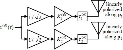
Figure 6: Model for the desired emitter’s transmit antenna.

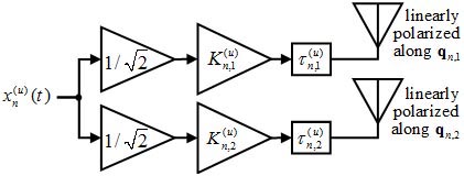
Figure 7: Model for the $n$th undesired emitter’s transmit antenna.

$K_1^{(d)}={\overline{K}}_1^{(d)}{K}^{(d)},$

(30)

$K_2^{(d)}={\overline{K}}_2^{(d)}{K}^{(d)},$

(31)

$\begin{array}{ccc}\hfill \tau {}_1^{(d)}& \hfill =\hfill & -\measuredangle [c_{{\alpha }^{(d)}}-s_{{\alpha }^{(d)}}{e}^{j{\delta }^{(d)}}/R^{(d)}]\mathrm{/}(2\pi f_{RF})\hfill \\ & & -r^{(d)}/c+k{}_1{}^{(d)}/f{}_{RF},\hfill \end{array}$

(32)

and

$\begin{array}{ccc}\hfill \tau {}_2^{(d)}& \hfill =\hfill & -\measuredangle [s_{{\alpha }^{(d)}}+c_{{\alpha }^{(d)}}{e}^{j{\delta }^{(d)}}/R^{(d)}]\mathrm{/}(2\pi f_{RF})\hfill \\ & & -r^{(d)}/c+k{}_2{}^{(d)}/f{}_{RF}.\hfill \end{array}$

(33)

In (30) and (31), respectively,

${\overline{K}}_1^{(d)}=\frac{\frac{1}{r^{(d)}}\sqrt{\frac{Z_0{G}^{(d)}}{2\pi }}\left|c_{{\alpha }^{(d)}}-\frac{s_{{\alpha }^{(d)}}{e}^{j{\delta }^{(d)}}}{R^{(d)}}\right|}{\sqrt{{\left|c_{{\alpha }^{(d)}}-\frac{s_{{\alpha }^{(d)}}{e}^{j{\delta }^{(d)}}}{R^{(d)}}\right|}^2+{\left|s_{{\alpha }^{(d)}}+\frac{c_{{\alpha }^{(d)}}{e}^{j{\delta }^{(d)}}}{R^{(d)}}\right|}^2}},$

(34)

and

${\overline{K}}_2^{(d)}=\frac{\frac{1}{r^{(d)}}\sqrt{\frac{Z_0{G}^{(d)}}{2\pi }}\left|s_{{\alpha }^{(d)}}+\frac{c_{{\alpha }^{(d)}}{e}^{j{\delta }^{(d)}}}{R^{(d)}}\right|}{\sqrt{{\left|c_{{\alpha }^{(d)}}-\frac{s_{{\alpha }^{(d)}}{e}^{j{\delta }^{(d)}}}{R^{(d)}}\right|}^2+{\left|s_{{\alpha }^{(d)}}+\frac{c_{{\alpha }^{(d)}}{e}^{j{\delta }^{(d)}}}{R^{(d)}}\right|}^2}}.$

(35)

In both (30) and (31),

$\begin{array}{ccc}\hfill K{}^{(d)}& \hfill =\hfill & \frac{A_s^{(d)}\lambda }{2}\sqrt{\frac{G^{(d)}}{Z_0\pi \left[{\left(E_1^{(d)}\right)}^2+{\left(E_2^{(d)}\right)}^2\right]}}\hfill \end{array},$

(36)

where [16] A${}_s$${}^{\mathrm{(}}$${}^d$${}^{\mathrm{)}}$ is the amplitude in volts of the monochromatic source signal which results in the amplitudes E${}_{\mathrm{1}}$${}^{\mathrm{(}}$${}^d$${}^{\mathrm{)}}$ and E${}_{\mathrm{2}}$${}^{\mathrm{(}}$${}^d$${}^{\mathrm{)}}$ of the spatially orthogonal electric-field components appearing at O. In (32) and (33), positive integers k${}_{\mathrm{1}}$${}^{\mathrm{(}}$${}^d$${}^{\mathrm{)}}$ and k${}_{\mathrm{2}}$${}^{\mathrm{(}}$${}^d$${}^{\mathrm{)}}$ respectively satisfy

$\begin{array}{c}\measuredangle \left[c_{{\alpha }^{(d)}}-s_{{\alpha }^{(d)}}{e}^{j{\delta }^{(d)}}/R^{(d)}\right]=\hfill \\ -2\pi f_{RF}{\tau }_1^{(d)}-2\pi f_{RF}{r}^{(d)}/c+2\pi k_1^{(d)}\hfill \end{array},$

(37)

and

$\begin{array}{c}\measuredangle \left[s_{{\alpha }^{(d)}}+c_{{\alpha }^{(d)}}{e}^{j{\delta }^{(d)}}/R^{(d)}\right]=\hfill \\ -2\pi f_{RF}{\tau }_2^{(d)}-2\pi f_{RF}{r}^{(d)}/c+2\pi k_2^{(d)}.\hfill \end{array}$

(38)

E. Electrical description of undesired emitters’ antennas

We assume the nth undesired emitter’s transmit antenna has a known total gain of G${}_n$${}^{\mathrm{(}}$${}^u$${}^{\mathrm{)}}$ in the direction of $O$. We further assume that, in the direction of $O$, the nth undesired emitter’s transmit antenna has a polarization characterized by axial ratio R${}_n$${}^{\mathrm{(}}$${}^u$${}^{\mathrm{)}}$, tilt angle $\alpha$${}_n$${}^{(}$${}^u$${}^{)}$, and rotation sense s${}_n$${}^{\mathrm{(}}$${}^u$${}^{\mathrm{)}}$. The phase difference $\delta$${}_n$${}^{(}$${}^u$${}^{)}$ between the untilted spatially orthogonal electric-field components appearing in the far field is [16]

${\delta }_n^{(u)}=\{\begin{array}{cc}\hfill -\pi /2,\hfill & \hfill s_n^{(u)}=R\hfill \\ \hfill \pi /2,\hfill & \hfill s_n^{(u)}=L\hfill \end{array}.$

(39)

Given these characteristics, we model the nth undesired emitter’s transmit antenna as shown in Figure 7,where [16]

$K_{n,1}^{(u)}={\overline{K}}_{n,1}^{(u)}{K}_n^{(u)},$

(40)

$K_{n,2}^{(u)}={\overline{K}}_{n,2}^{(u)}{K}_n^{(u)},$

(41)

$\begin{array}{ccc}\hfill {\tau }_{n,1}^{(u)}& \hfill =\hfill & -\measuredangle [c_{{\alpha }_n^{(u)}}-s_{{\alpha }_n^{(u)}}{e}^{j{\delta }_n^{(u)}}/R_n^{(u)}]\mathrm{/}(2\pi f_{RF})\hfill \\ & & -r_n^{(u)}/c+k{}_{n,1}{}^{(u)}/f{}_{RF},\hfill \end{array}$

(42)

and

$\begin{array}{ccc}\hfill \tau {}_{n,2}^{(u)}& \hfill =\hfill & -\measuredangle [s_{{\alpha }_n^{(u)}}+c_{{\alpha }_n^{(u)}}{e}^{j{\delta }_n^{(u)}}/R_n^{(u)}]\mathrm{/}(2\pi f_{RF})\hfill \\ & & -r_n^{(u)}/c+k{}_{n,2}{}^{(u)}/f{}_{RF}.\hfill \end{array}$

(43)

In (40) and (41), respectively,

${\overline{K}}_{n,1}^{(u)}=\frac{\frac{1}{r_n^{(u)}}\sqrt{\frac{Z_0{G}_n^{(u)}}{2\pi }}\left|c_{{\alpha }_n^{(u)}}-\frac{s_{{\alpha }_n^{(u)}}{e}^{j{\delta }_n^{(u)}}}{R_n^{(u)}}\right|}{\sqrt{{\left|c_{{\alpha }_n^{(u)}}-\frac{s_{{\alpha }_n^{(u)}}{e}^{j{\delta }_n^{(u)}}}{R_n^{(u)}}\right|}^2+{\left|s_{{\alpha }_n^{(u)}}+\frac{c_{{\alpha }_n^{(u)}}{e}^{j{\delta }_n^{(u)}}}{R_n^{(u)}}\right|}^2}},$

(44)

and

${\overline{K}}_{n,2}^{(u)}=\frac{\frac{1}{r_n^{(u)}}\sqrt{\frac{Z_0{G}_n^{(u)}}{2\pi }}\left|s_{{\alpha }_n^{(u)}}+\frac{c_{{\alpha }_n^{(u)}}{e}^{j{\delta }_n^{(u)}}}{R_n^{(u)}}\right|}{\sqrt{{\left|c_{{\alpha }_n^{(u)}}-\frac{s_{{\alpha }_n^{(u)}}{e}^{j{\delta }_n^{(u)}}}{R_n^{(u)}}\right|}^2+{\left|s_{{\alpha }_n^{(u)}}+\frac{c_{{\alpha }_n^{(u)}}{e}^{j{\delta }_n^{(u)}}}{R_n^{(u)}}\right|}^2}}.$

(45)

In both (40) and (41),

$K_n^{(u)}=\frac{A_{n,s}^{(u)}\lambda }{2}\sqrt{\frac{G_n^{(u)}}{\pi Z_0\left[{\left(E_{n,1}^{(u)}\right)}^2+{\left(E_{n,2}^{(u)}\right)}^2\right]}}=\frac{\lambda r_n^{(u)}}{Z_0},$

(46)

where [16] A${}_n$${}_{\mathrm{,}}$${}_s$${}^{\mathrm{(}}$${}^u$${}^{\mathrm{)}}$ is the amplitude in volts of the monochromatic source signal which results in the amplitudes E${}_n$${}_{\mathrm{,}\mathrm{1}}$${}^{\mathrm{(}}$${}^u$${}^{\mathrm{)}}$ and E${}_n$${}_{\mathrm{,}\mathrm{2}}$${}^{\mathrm{(}}$${}^u$${}^{\mathrm{)}}$ of the spatially orthogonal electric-field components appearing at O. In (42) and (43), positive integers k${}_n$${}_{\mathrm{,}\mathrm{1}}$${}^{\mathrm{(}}$${}^u$${}^{\mathrm{)}}$ and k${}_n$${}_{\mathrm{,}\mathrm{2}}$${}^{\mathrm{(}}$${}^u$${}^{\mathrm{)}}$ respectively satisfy

$\begin{array}{c}\measuredangle \left[c_{{\alpha }_n^{(u)}}-s_{{\alpha }_n^{(u)}}{e}^{j{\delta }_n^{(u)}}/R_n^{(u)}\right]=\hfill \\ -2\pi f_{RF}{\tau }_{n,1}^{(u)}-2\pi f_{RF}{r}_n^{(u)}/c+2\pi k_{n,1}^{(u)}\hfill \end{array},$

(47)

and

$\begin{array}{c}\measuredangle \left[s_{{\alpha }_n^{(u)}}+c_{{\alpha }_n^{(u)}}{e}^{j{\delta }_n^{(u)}}/R_n^{(u)}\right]=\hfill \\ -2\pi f_{RF}{\tau }_{n,2}^{(u)}-2\pi f_{RF}{r}_n^{(u)}/c+2\pi k_{n,2}^{(u)}.\hfill \end{array}$

(48)

F. Electric fields incident on antenna array’s elements

Since the desired emitter’s transmitter sends (16) to its antenna, the desired emitter’s antenna effectively produces at a point very near D on the line passing through D and O the vector electric field [16]

$\begin{array}{c}{𝐄}_D^{(d)}(t)\approx \hfill \\ \frac{K_1^{(d)}{A}^{(d)}(t)}{\sqrt{2}}\cos \left[2\pi f_{RF}(t-{\tau }_1^{(d)})+{\gamma }^{(d)}(t)\right]{𝐩}_1\hfill \\ +\frac{K_2^{(d)}{A}^{(d)}(t)}{\sqrt{2}}\cos \left[2\pi f_{RF}(t-{\tau }_2^{(d)})+{\gamma }^{(d)}(t)\right]{𝐩}_2.\hfill \end{array}$

(49)

After propagating to the receive-antenna array’s mth element’s pth port’s phase center, the desired emitter’s transmitted electric field is

$\begin{array}{c}{𝐄}_{m,p}^{(d)}(t)\approx -{\overline{K}}_1^{(d)}{A}^{(d)}(t-{\tau }^{(d)})/\sqrt{2}\hfill \\ \times \cos \left[2\pi f_{RF}(t-{\tau }_1^{(d)}-{\tau }_{m,p}^{d\to a})+{\gamma }^{(d)}(t-{\tau }^{(d)})\right]{𝐚}_1\hfill \\ +{\overline{K}}_2^{(d)}{A}^{(d)}(t-{\tau }^{(d)})/\sqrt{2}\hfill \\ \times \cos \left[2\pi f_{RF}(t-{\tau }_2^{(d)}-{\tau }_{m,p}^{d\to a})+{\gamma }^{(d)}(t-{\tau }^{(d)})\right]{𝐚}_2,\hfill \end{array}$

(50)

where

${\tau }^{(d)}=r^{(d)}/c,$

(51)

is the propagation delay from D to O and

$\begin{array}{c}{\tau }_{m,p}^{(d\to a)}=r_{m,p}^{(d\to a)}/c\approx r^{(d)}/c\hfill \\ -\left[s_{{\theta }^{(d)}}{c}_{{\varphi }^{(d)}}{x}_{m,p}^{(a)}+s_{{\theta }^{(d)}}{s}_{{\varphi }^{(d)}}{y}_{m,p}^{(a)}+c_{{\theta }^{(d)}}{z}_{m,p}^{(a)}\right]\mathrm{/}c\hfill \end{array},$

(52)

is the propagation delay from D to the phase center of the receive-antenna array’s mth element’s pth port.

Since the nth undesired emitter’s transmitter sends (18) to its antenna, the nth undesired emitter’s antenna produces at a point very near $U_n$ on the line passing through U${}_n$ and O the vector electric field [16]

$\begin{array}{c}{𝐄}_{n\to U_n}^{(u)}(t)\approx K_{n,1}^{(u)}{A}_n^{(u)}(t)/\sqrt{2}\hfill \\ \times \cos \left[2\pi f_{RF}(t-{\tau }_{n,1}^{(u)})+{\gamma }_n^{(u)}(t)\right]{𝐪}_{n,1}\hfill \\ +K_{n,2}^{(u)}{A}_n^{(u)}(t)/\sqrt{2}\hfill \\ \times \cos \left[2\pi f_{RF}(t-{\tau }_{n,2}^{(u)})+{\gamma }_n^{(u)}(t)\right]{𝐪}_{n,2}.\hfill \end{array}$

(53)

After propagating to the receive-antenna array’s mth element’s pth port’s phase center, the nth undesired emitter’s transmitted electric field is

$\begin{array}{c}{𝐄}_{n\to m,p}^{(u)}(t)\approx -{𝐮}_{n,1}{\overline{K}}_{n,1}^{(u)}{A}_n^{(u)}(t-{\tau }_n^{(u)})/\sqrt{2}\hfill \\ \times \cos \left[2\pi f_{RF}(t-{\tau }_{n,1}^{(u)}-{\tau }_{n\to m,p}^{(u\to a)})+{\gamma }_n^{(u)}(t-{\tau }_n^{(u)})\right]\hfill \\ +{𝐮}_{n,2}{\overline{K}}_2^{(u,n)}{A}_n^{(u)}(t-{\tau }_n^{(u)})/\sqrt{2}\hfill \\ \times \cos \left[2\pi f_{RF}(t-{\tau }_{n,2}^{(u)}-{\tau }_{n\to m,p}^{(u\to a)})+{\gamma }_n^{(u)}(t-{\tau }_n^{(u)})\right],\hfill \end{array}$

(54)

where

${\tau }_n^{(u)}=r_n^{(u)}/c,$

(55)

is the propagation delay from U${}_n$ to O and

$\begin{array}{c}{\tau }_{n\to m,p}^{(u\to a)}=r_{n\to m,p}^{(u\to a)}/c\approx r_n^{(u)}/c\hfill \\ -\frac{s_{{\theta }_n^{(u)}}{c}_{{\varphi }_n^{(u)}}{x}_{m,p}^{(a)}+s_{{\theta }_n^{(u)}}{s}_{{\varphi }_n^{(u)}}{y}_{m,p}^{(a)}+c_{{\theta }_n^{(u)}}{z}_{m,p}^{(a)}}{c}\hfill \end{array},$

(56)

is the propagation delay from U${}_n$ to the phase center of the receive-antenna array’s mth element’s pth port.

G. Output signals of receive-antenna array’s elements

We assume the ports of the receive-antenna array’s elements respond linearly to incident EM waves. That is, each port’s response to the incident EM waves from the desired and undesired emitters is the sum of that port’s response to the individual incident EM waves. We further assume mutually independent thermal-noise signals corrupt the array’s 2M outputs.

The response of the receive-antenna array’s mth element’s pth port to (50) is

$\begin{array}{c}{x}_{m,p}^{(d)}(t)\approx -K_{m,p,1}^{(a)}({\theta }^{(d)},{\varphi }^{(d)}){\overline{K}}_1^{(d)}{A}^{(d)}(t-{\tau }^{(d)})/2\hfill \\ \times \cos \{2\pi f_{RF}[t-{\tau }_1^{(d)}-{\tau }_{m,p}^{{}_{(d\to a)}}-{\tau }_{m,p,1}^{{}_{(a)}}({\theta }^{(d)},{\varphi }^{(d)})]\hfill \\ +{\gamma }^{(d)}(t-{\tau }^{(d)})\}\hfill \\ +K_{m,p,2}^{(a)}({\theta }^{(d)},{\varphi }^{(d)}){\overline{K}}_2^{(d)}{A}^{(d)}(t-{\tau }^{(d)})/2\hfill \\ \times \cos \{2\pi f_{RF}[t-{\tau }_2^{(d)}-{\tau }_{m,p}^{{}_{(d\to a)}}-{\tau }_{m,p,2}^{{}_{(a)}}({\theta }^{(d)},{\varphi }^{(d)})]\hfill \\ +{\gamma }^{(d)}(t-{\tau }^{(d)})\}.\hfill \end{array}$

(57)

The response of the receive-antenna array’s mth element’s pth port to (54) is

$\begin{array}{c}{x}_{m,p}^{(u,n)}(t)\approx \hfill \\ -\left[K_{m,p,1}^{(a)}({\theta }_n^{(u)},{\varphi }_n^{(u)}){\overline{K}}_{n,1}^{(u)}/2\right]A_n^{(u)}(t-{\tau }_n^{(u)})\hfill \\ \times \cos \{2\pi f_{RF}[t-{\tau }_{n,1}^{(u)}-{\tau }_{n\to m,p}^{(u\to a)}-{\tau }_{m,p,1}^{(a)}({\theta }_n^{(u)},{\varphi }_n^{(u)})]\hfill \\ +{\gamma }_n^{(u)}(t-{\tau }_n^{(u)})\}\hfill \\ +\left[K_{m,p,2}^{(a)}({\theta }_n^{(u)},{\varphi }_n^{(u)}){\overline{K}}_{n,2}^{(u)}/2\right]A_n^{(u)}(t-{\tau }_n^{(u)})\hfill \\ \times \cos \{2\pi f_{RF}[t-{\tau }_{n,2}^{(u)}-{\tau }_{n\to m,p}^{(u\to a)}-{\tau }_{m,p,2}^{(a)}({\theta }_n^{(u)},{\varphi }_n^{(u)})]\hfill \\ +{\gamma }_n^{(u)}(t-{\tau }_n^{(u)})\}.\hfill \end{array}$

(58)

WSS, Gaussian, zero-mean thermal-noise signal

$\begin{array}{ccc}\hfill x{}_{m,p}{}^{(tn)}(t)& \hfill =\hfill & x_{I,m,p}^{(tn)}(t)\cos (2\pi f_{RF}t)\hfill \\ & & -x_{Q,m,p}^{(tn)}(t)\sin (2\pi f{}_{RF}t)\hfill \end{array},$

(59)

additively corrupts the output of the pth port of the mth antenna-array element. In (59) x${}_I$${}_{\mathrm{,}m\mathrm{,}p}$${}^{\mathrm{(}}$${}^{t\mathit{}n}$${}^{\mathrm{)}}$(t) and x${}_Q$${}_{\mathrm{,}m\mathrm{,}p}$${}^{\mathrm{(}}$${}^t$${}^n$${}^{\mathrm{)}}$(t) are, respectively, the I and Q components of x${}_{m\mathrm{,}p}$${}^{\mathrm{(}}$${}^{t\mathit{}n}$${}^{\mathrm{)}}$(t). The thermal-noise signal has PSD

$S_{m,p}^{(tn)}(f)=\frac{N_{m,p}^{(tn)}}{2}\left[\mathrm{\Pi }\left(\frac{f-f_{RF}}{B_{m,p}^{(tn)}}\right)+\mathrm{\Pi }\left(\frac{f+f_{RF}}{B_{m,p}^{(tn)}}\right)\right],$

(60)

where N${}_m$${}_{\mathrm{,}}$${}_p$${}^{\mathrm{(}}$${}^{t\mathit{}n}$${}^{\mathrm{)}}$/2 is the PSD’s level in W/Hz and B${}_m$${}_{\mathrm{,}}$${}_p$${}^{\mathrm{(}}$${}^{t\mathit{}n}$${}^{\mathrm{)}}$ is the RF bandwidth in Hz of the thermal noise of the pth port of the mth antenna-array element. The I and Q thermal-noise components of the pth port of the mth antenna-array element are independent, zero-mean, Gaussian, WSS random lowpass processes with PSD

$S_{I,m,p}^{(tn)}(f)=S_{Q,m,p}^{(tn)}(f)=N_{m,p}^{(tn)}\mathrm{\Pi }\left[f/B_{m,p}^{(tn)}\right].$

(61)

H. Receiver/spatial-processor model

Figure 8 shows the 2M ports’ output signals feeding the employed receiver/spatial-processor model. Phase-synchronized quadrature demodulators [17] linearly produce the complex envelopes of their respective inputs. Samplers then take time-coincident samples of these complex envelopes, and the weight-and-sum network produces a weighted sum of the 2M sampled values. The model of Figure 8 represents several practical systems. For example, this model represents a system which scales in amplitude and shifts in phase 2M RF signals prior to summing them to produce a single RF signal which then feeds, e.g., a global navigation satellite system (GNSS) receiver or a single GNSS-receiver channel (i.e., a channel corresponding to a specific GNSS satellite’s unique pseudorandom-noise code).

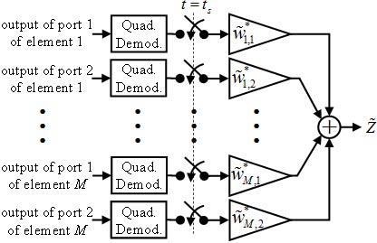
Figure 8: Receiver/spatial-processor model.

The complex envelope of (57) is

${\tilde{x}}_{m,p}^{(d)}(t)\approx {\tilde{d}}_{m,p}{A}^{(d)}(t-{\tau }^{(d)})e^{j{\gamma }^{(d)}(t-{\tau }^{(d)})},$

(62)

where

$\begin{array}{c}{\tilde{d}}_{m,p}=-K_{m,p,1}^{(a)}({\theta }^{(d)},{\varphi }^{(d)}){\overline{K}}_1^{(d)}\mathrm{/}2\hfill \\ \times e^{-j2\pi f_{RF}[{\tau }_1^{(d)}+{\tau }_{m,p}^{{}_{(d\to a)}}+{\tau }_{m,p,1}^{{}_{(a)}}({\theta }^{(d)},{\varphi }^{(d)})]}\hfill \\ +K_{m,p,2}^{(a)}({\theta }^{(d)},{\varphi }^{(d)}){\overline{K}}_2^{(d)}\mathrm{/}2\hfill \\ \times e^{-j2\pi f_{RF}[{\tau }_2^{(d)}+{\tau }_{m,p}^{{}_{(d\to a)}}+{\tau }_{m,p,2}^{{}_{(a)}}({\theta }^{(d)},{\varphi }^{(d)})]}\hfill \\ =e^{-j2\pi f_{RF}{\tau }_{m,p}^{d\to a}}\hfill \\ \times \{-K_{m,p,1}^{(a)}({\theta }^{(d)},{\varphi }^{(d)}){\overline{K}}_1^{(d)}\mathrm{/}2\hfill \\ \times e^{-j2\pi f_{RF}\left[{\tau }_1^{(d)}+{\tau }_{m,p,1}^{(a)}({\theta }^{(d)},{\varphi }^{(d)})\right]}\hfill \\ +K_{m,p,2}^{(a)}({\theta }^{(d)},{\varphi }^{(d)}){\overline{K}}_2^{(d)}\mathrm{/}2\hfill \\ \times e^{-j2\pi f_{RF}\left[{\tau }_2^{(d)}+{\tau }_{m,p,2}^{(a)}({\theta }^{(d)},{\varphi }^{(d)})\right]}\}\hfill \\ \approx e^{-j2\pi f_{RF}\left[\frac{r^{(d)}-s_{{\theta }^{(d)}}{c}_{{\varphi }^{(d)}}{x}_{m,p}^{(a)}-s_{{\theta }^{(d)}}{s}_{{\varphi }^{(d)}}{y}_{m,p}^{(a)}-c_{{\theta }^{(d)}}{z}_{m,p}^{(a)}}{c}\right]}\hfill \\ \times \{-K_{m,p,1}^{(a)}({\theta }^{(d)},{\varphi }^{(d)}){\overline{K}}_1^{(d)}\mathrm{/}2\hfill \\ \times e^{-j2\pi f_{RF}\left[{\tau }_1^{(d)}+{\tau }_{m,p,1}^{(a)}({\theta }^{(d)},{\varphi }^{(d)})\right]}\hfill \\ +K_{m,p,2}^{(a)}({\theta }^{(d)},{\varphi }^{(d)}){\overline{K}}_2^{(d)}\mathrm{/}2\hfill \\ \times e^{-j2\pi f_{RF}\left[{\tau }_2^{(d)}+{\tau }_{m,p,2}^{(a)}({\theta }^{(d)},{\varphi }^{(d)})\right]}\}.\hfill \end{array}$

(63)

For future convenience we define

$\begin{array}{c}{\tilde{g}}_{m,p}=e^{-j2\pi f_{RF}\left[\frac{-s_{{\theta }^{(d)}}{c}_{{\varphi }^{(d)}}{x}_{m,p}^{(a)}-s_{{\theta }^{(d)}}{s}_{{\varphi }^{(d)}}{y}_{m,p}^{(a)}-c_{{\theta }^{(d)}}{z}_{m,p}^{(a)}}{c}\right]}\hfill \\ \times \{-K_{m,p,1}^{(a)}({\theta }^{(d)},{\varphi }^{(d)}){\overline{K}}_1^{(d)}\mathrm{/}2\hfill \\ \times e^{-j2\pi f_{RF}\left[{\tau }_1^{(d)}+{\tau }_{m,p,1}^{(a)}({\theta }^{(d)},{\varphi }^{(d)})\right]}\hfill \\ +K_{m,p,2}^{(a)}({\theta }^{(d)},{\varphi }^{(d)}){\overline{K}}_2^{(d)}\mathrm{/}2\hfill \\ \times e^{-j2\pi f_{RF}\left[{\tau }_2^{(d)}+{\tau }_{m,p,2}^{(a)}({\theta }^{(d)},{\varphi }^{(d)})\right]}\}\hfill \\ \Rightarrow {\tilde{d}}_{m,p}\approx e^{-j2\pi f_{RF}{r}^{(d)}/c}{\tilde{g}}_{m,p}.\hfill \end{array}$

(64)

The complex envelope of (58) is

$\begin{array}{c}{\tilde{x}}_{m,p}^{(u,n)}(t)\approx {\tilde{u}}_{n,m,p}{A}_n^{(u)}(t-{\tau }_n^{(u)})e^{j{\gamma }_n^{(u)}(t-{\tau }_n^{(u)})}\hfill \\ ={\tilde{u}}_{n,m,p}\left[x_{I,n}^{(u)}(t-{\tau }_n^{(u)})+j{x}_{Q,n}^{(u)}(t-{\tau }_n^{(u)})\right],\hfill \end{array}$

(65)

where

$\begin{array}{c}{\tilde{u}}_{n,m,p}=-K_{m,p,1}^{(a)}({\theta }_n^{(u)},{\varphi }_n^{(u)}){\overline{K}}_{n,1}^{(u)}/2\hfill \\ \times e^{-j2\pi f_{RF}\left[{\tau }_{n,1}^{(u)}+{\tau }_{n\to m,p}^{(u\to a)}+{\tau }_{m,p,1}^{{}_{(a)}}({\theta }_n^{(u)},{\varphi }_n^{(u)})\right]}\hfill \\ +K_{m,p,2}^{(a)}({\theta }_n^{(u)},{\varphi }_n^{(u)}){\overline{K}}_{n,2}^{(u)}/2\hfill \\ \times e^{-j2\pi f_{RF}\left[{\tau }_{n,2}^{(u)}+{\tau }_{n\to m,p}^{(u\to a)}+{\tau }_{m,p,2}^{{}_{(a)}}({\theta }_n^{(u)},{\varphi }_n^{(u)})\right]}\hfill \\ =e^{-j2\pi f_{RF}{\tau }_{n\to m,p}^{(u\to a)}}[-K_{m,p,1}^{(a)}({\theta }_n^{(u)},{\varphi }_n^{(u)}){\overline{K}}_{n,1}^{(u)}/2\hfill \\ \times e^{-j2\pi f_{RF}\left[{\tau }_{n,1}^{(u)}+{\tau }_{m,p,1}^{(a)}({\theta }_n^{(u)},{\varphi }_n^{(u)})\right]}\hfill \\ +K_{m,p,2}^{(a)}({\theta }_n^{(u)},{\varphi }_n^{(u)}){\overline{K}}_{n,2}^{(u)}/2\hfill \\ \times e^{-j2\pi f_{RF}\left[{\tau }_{n,2}^{(u)}+{\tau }_{m,p,2}^{(a)}({\theta }_n^{(u)},{\varphi }_n^{(u)})\right]}]\hfill \\ \approx e^{-j2\pi f_{RF}\left[\frac{r_n^{(u)}-s_{{\theta }_n^{(u)}}{c}_{{\varphi }_n^{(u)}}{x}_{m,p}^{(a)}-s_{{\theta }_n^{(u)}}{s}_{{\varphi }_n^{(u)}}{y}_{m,p}^{(a)}-c_{{\theta }_n^{(u)}}{z}_{m,p}^{(a)}}{c}\right]}\hfill \\ \times [-K_{m,p,1}^{(a)}({\theta }_n^{(u)},{\varphi }_n^{(u)}){\overline{K}}_{n,1}^{(u)}/2\hfill \\ \times e^{-j2\pi f_{RF}\left[{\tau }_{n,1}^{(u)}+{\tau }_{m,p,1}^{(a)}({\theta }_n^{(u)},{\varphi }_n^{(u)})\right]}\hfill \\ +K_{m,p,2}^{(a)}({\theta }_n^{(u)},{\varphi }_n^{(u)}){\overline{K}}_{n,2}^{(u)}/2\hfill \\ \times e^{-j2\pi f_{RF}\left[{\tau }_{n,2}^{(u)}+{\tau }_{m,p,2}^{(a)}({\theta }_n^{(u)},{\varphi }_n^{(u)})\right]}].\hfill \end{array}$

(66)

For future convenience we define

$\begin{array}{c}{\tilde{h}}_{n,m,p}=\hfill \\ e^{-j2\pi f_{RF}\left[\frac{-s_{{\theta }_n^{(u)}}{c}_{{\varphi }_n^{(u)}}{x}_{m,p}^{(a)}-s_{{\theta }_n^{(u)}}{s}_{{\varphi }_n^{(u)}}{y}_{m,p}^{(a)}-c_{{\theta }_n^{(u)}}{z}_{m,p}^{(a)}}{c}\right]}\hfill \\ \times [-K_{m,p,1}^{(a)}({\theta }_n^{(u)},{\varphi }_n^{(u)}){\overline{K}}_{n,1}^{(u)}/2\hfill \\ \times e^{-j2\pi f_{RF}\left[{\tau }_{n,1}^{(u)}+{\tau }_{m,p,1}^{(a)}({\theta }_n^{(u)},{\varphi }_n^{(u)})\right]}\hfill \\ +K_{m,p,2}^{(a)}({\theta }_n^{(u)},{\varphi }_n^{(u)}){\overline{K}}_{n,2}^{(u)}/2\hfill \\ \times e^{-j2\pi f_{RF}\left[{\tau }_{n,2}^{(u)}+{\tau }_{m,p,2}^{(a)}({\theta }_n^{(u)},{\varphi }_n^{(u)})\right]}]\hfill \\ \Rightarrow {\tilde{u}}_{n,m,p}\approx e^{-j2\pi f_{RF}{r}_n^{(u)}/c}{\tilde{h}}_{n,m,p}.\hfill \end{array}$

(67)

The complex envelope of (59) is

${\tilde{x}}_{m,p}^{(tn)}(t)=x_{I,m,p}^{(tn)}(t)+j{x}_{Q,m,p}^{(tn)}(t).$

(68)

The component of the sampled complex envelope of themth element’s pth port’s output due to the desired emitter’s signal is

$\begin{array}{c}{\tilde{x}}_{m,p}^{(d)}(t_s)={\tilde{X}}_{m,p}^{(d)}\hfill \\ \approx {\tilde{d}}_{m,p}{A}^{(d)}(t_s-{\tau }^{(d)})e^{j{\gamma }^{(d)}(t_s-{\tau }^{(d)})}.\hfill \end{array}$

(69)

The component of the sampled complex envelope of themth element’s pth port’s output due to the nth undesired emitter’s signal is

$\begin{array}{c}{\tilde{x}}_{m,p}^{(u,n)}(t_s)={\tilde{X}}_{m,p}^{(u,n)}\hfill \\ \approx {\tilde{u}}_{n,m,p}\left[x_{I,n}^{(u)}(t_s-{\tau }_n^{(u)})+j{x}_{Q,n}^{(u)}(t_s-{\tau }_n^{(u)})\right].\hfill \end{array}$

(70)

The component of the sampled complex envelope of the mth element’s pth port’s output due to thermal noise is

$\begin{array}{c}{\tilde{x}}_{m,p}^{(tn)}(t_s)={\tilde{X}}_{m,p}^{(tn)}\hfill \\ =x_{I,m,p}^{(tn)}(t_s)+j{x}_{Q,m,p}^{(tn)}(t_s)=X_{I,m,p}^{(tn)}+j{X}_{Q,m,p}^{(tn)}.\hfill \end{array}$

(71)

The receiver/spatial processor’s final output is

$\tilde{Z}=\sum _{p=1}^2\sum _{m=1}^M{\tilde{w}}_{m,p}^{*}\left[{\tilde{X}}_{m,p}^{(d)}+\sum _{n=1}^N{\tilde{X}}_{n,m,p}^{(u)}+{\tilde{X}}_{m,p}^{(tn)}\right].$

(72)

The component of the receiver/spatial processor’s final output due to the desired emitter’s signal is

$\begin{array}{c}\tilde{S}=\sum _{p=1}^2\sum _{m=1}^M{\tilde{w}}_{m,p}^{*}{\tilde{X}}_{m,p}^{(d)}\hfill \\ \approx A^{(d)}(t_s-{\tau }^{(d)})e^{j{\gamma }^{(d)}(t_s-{\tau }^{(d)})}\sum _{p=1}^2\sum _{m=1}^M{\tilde{w}}_{m,p}^{*}{\tilde{d}}_{m,p}.\hfill \end{array}$

(73)

The component of the receiver/spatial processor’s final output due to the N undesired emitters’ signals is

$\begin{array}{c}\tilde{U}=\sum _{p=1}^2\sum _{m=1}^M{\tilde{w}}_{m,p}^{*}\sum _{n=1}^N{\tilde{X}}_{n,m,p}^{(u)}=\sum _{n=1}^N\sum _{p=1}^2\sum _{m=1}^M{\tilde{w}}_{m,p}^{*}{\tilde{X}}_{n,m,p}^{(u)}\hfill \\ \approx \sum _{n=1}^N\left[x_{I,n}^{(u)}(t_s-{\tau }_n^{(u)})+j{x}_{Q,n}^{(u)}(t_s-{\tau }_n^{(u)})\right]\hfill \\ \times \sum _{p=1}^2\sum _{m=1}^M{\tilde{w}}_{m,p}^{*}{\tilde{u}}_{n,m,p}.\hfill \end{array}$

(74)

The component of the receiver/spatial processor’s final output due to the 2M thermal-noise signals is

$\begin{array}{cc}\hfill \tilde{N}& =\sum _{p=1}^2\sum _{m=1}^M{\tilde{w}}_{m,p}^{*}{\tilde{X}}_{m,p}^{(tn)}\hfill \\ & =\sum _{p=1}^2\sum _{m=1}^M{\tilde{w}}_{m,p}^{*}\left[X_{I,m,p}^{(tn)}+j{X}_{Q,m,p}^{(tn)}\right].\hfill \end{array}$

(75)

I. Problem statement

We define the SIR as [12]

$SIR\stackrel{\mathrm{\Delta }}{=}\frac{{\left|\tilde{S}\right|}^2}{E\left[{\left|\tilde{U}+\tilde{N}\right|}^2\right]},$

(76)

where E($\cdot$) denotes expectation. We desire to maximize (76) by choosing

$𝐰={\left[\begin{array}{ccccc}\hfill {\tilde{w}}_{1,1}\hfill & \hfill {\tilde{w}}_{1,2}\hfill & \hfill \mathrm{\cdots }\hfill & \hfill {\tilde{w}}_{M,1}\hfill & \hfill {\tilde{w}}_{M,2}\hfill \end{array}\right]}^T$

(77)

subject to the traditional and practical constraint [12]

${𝐰}^{\prime }𝐰=1,$

(78)

where the ${}^{\prime }$ represents conjugated matrix transposition.

III. ALGORITHM GENERALIZATION

This section generalizes the spatial-processing algorithm of [1] to support arrays of dual-polarization antenna elements. The squared magnitude of (73) is

$\begin{array}{c}{\left|\tilde{S}\right|}^2\approx {\left[A^{(d)}(t_s-{\tau }^{(d)})\right]}^2{\left|\sum _{p=1}^2\sum _{m=1}^M{\tilde{w}}_{m,p}^{*}{\tilde{d}}_{m,p}\right|}^2\hfill \\ \approx {\left[A^{(d)}(t_s-{\tau }^{(d)})\right]}^2{\left|\sum _{p=1}^2\sum _{m=1}^M{\tilde{w}}_{m,p}^{*}{e}^{-j2\pi f_{RF}{r}^{(d)}/c}{\tilde{g}}_{m,p}\right|}^2\hfill \\ ={\left[A^{(d)}(t_s-{\tau }^{(d)})\right]}^2{\left|\sum _{p=1}^2\sum _{m=1}^M{\tilde{w}}_{m,p}^{*}{\tilde{g}}_{m,p}\right|}^2.\hfill \end{array}$

(79)

By defining a second complex vector

$𝐬={\left[\begin{array}{ccccc}\hfill {\tilde{g}}_{1,1}\hfill & \hfill {\tilde{g}}_{1,2}\hfill & \hfill \mathrm{\cdots }\hfill & \hfill {\tilde{g}}_{M,1}\hfill & \hfill {\tilde{g}}_{M,2}\hfill \end{array}\right]}^T,$

(80)

we can write (79) as

${\left|\tilde{S}\right|}^2\approx {\left[A^{(d)}(t_s-{\tau }^{(d)})\right]}^2{\left|{𝐰}^{\prime }𝐬\right|}^2.$

(81)

Since the 2M thermal-noise signals and the N undesired emitters’ signals are zero mean and mutually uncorrelated,

$\begin{array}{ccc}\hfill E\left[{\left|\tilde{U}+\tilde{N}\right|}^2\right]& \hfill =\hfill & E\left[\left(\tilde{U}+\tilde{N}\right){\left(\tilde{U}+\tilde{N}\right)}^{*}\right]\hfill \\ & \hfill =\hfill & E\left[{\left|\tilde{U}\right|}^2+\tilde{U}{\tilde{N}}^{*}+\tilde{N}{\tilde{U}}^{*}+{\left|\tilde{N}\right|}^2\right]\hfill \\ & \hfill =\hfill & E\left[{\left|\tilde{U}\right|}^2\right]+E\left[{\left|\tilde{N}\right|}^2\right],\hfill \end{array}$

(82)

so

$SIR={\left|\tilde{S}\right|}^2\mathrm{/}\left\{E\left[{\left|\tilde{U}\right|}^2\right]+E\left[{\left|\tilde{N}\right|}^2\right]\right\}.$

(83)

Now,

$\begin{array}{c}E\left[{\left|\tilde{N}\right|}^2\right]=E\left[{\left|\sum _{p=1}^2\sum _{m=1}^M{\tilde{w}}_{m,p}^{*}\left[X_{I,m,p}^{(tn)}+j{X}_{Q,m,p}^{(tn)}\right]\right|}^2\right]\hfill \\ =E\{\left[\sum _{p=1}^2\sum _{m=1}^M{\tilde{w}}_{m,p}^{*}[X_{I,m,p}^{(tn)}+j{X}_{Q,m,p}^{(tn)}]\right]\hfill \\ \times \left[\sum _{p=1}^2\sum _{m=1}^M{\tilde{w}}_{m,p}[X_{I,m,p}^{(tn)}-j{X}_{Q,m,p}^{(tn)}]\right]\}\hfill \\ =E\{\sum _{p=1}^2\sum _{q=1}^2\sum _{m=1}^M\sum _{l=1}^M{\tilde{w}}_{m,p}^{*}[X_{I,m,p}^{(tn)}+j{X}_{Q,m,p}^{(tn)}]\hfill \\ \times {\tilde{w}}_{l,q}[X_{I,l,q}^{(tn)}-j{X}_{Q,l,q}^{(tn)}]\}\hfill \\ =\sum _{p=1}^2\sum _{q=1}^2\sum _{m=1}^M\sum _{l=1}^M{\tilde{w}}_{m,p}^{*}{\tilde{w}}_{l,q}\{E\left[X_{I,m,p}^{(tn)}{X}_{I,l,q}^{(tn)}\right]\hfill \\ +E\left[X_{Q,m,p}^{(tn)}{X}_{Q,l,q}^{(tn)}\right]\}\hfill \\ =\sum _{p=1}^2\sum _{q=1}^2\sum _{m=1}^M\sum _{l=1}^M{\tilde{w}}_{m,p}^{*}{\tilde{w}}_{l,q}\left\{2N_{m,p}^{(tn)}{B}_{m,p}^{(tn)}{\delta }_{m,l}{\delta }_{p,q}\right\}\hfill \\ =2\sum _{p=1}^2\sum _{q=1}^2\sum _{m=1}^M{N}_{m,p}^{(tn)}{B}_{m,p}^{(tn)}{\tilde{w}}_{m,p}^{*}{\tilde{w}}_{m,q}{\delta }_{p,q}\hfill \\ =2\sum _{p=1}^2\sum _{m=1}^M{N}_{m,p}^{(tn)}{B}_{m,p}^{(tn)}{\left|{\tilde{w}}_{m,p}\right|}^2,\hfill \end{array}$

(84)

where $\delta$${}_m$${}_{,}$${}_l$ represents the Kronecker delta function, having a value of unity if m = l and zero otherwise. We next write

$\begin{array}{c}E\left[{\left|\tilde{U}\right|}^2\right]=E\left(\tilde{U}{\tilde{U}}^{*}\right)\hfill \\ \approx E\{\{\sum _{n=1}^N[x_{I,n}^{(u)}(t_s-{\tau }_n^{(u)})+j{x}_{Q,n}^{(u)}(t_s-{\tau }_n^{(u)})]\hfill \\ \times \left(\sum _{p=1}^2\sum _{m=1}^M{\tilde{w}}_{m,p}^{*}{\tilde{u}}_{n,m,p}\right)\}\hfill \\ \times \{\sum _{n=1}^N[x_{I,n}^{(u)}(t_s-{\tau }_n^{(u)})-j{x}_{Q,n}^{(u)}(t_s-{\tau }_n^{(u)})]\hfill \\ \times \left(\sum _{p=1}^2\sum _{m=1}^M{\tilde{w}}_{m,p}{\tilde{u}}_{n,m,p}^{*}\right)\}\}\hfill \\ =E\{\sum _{n=1}^N\sum _{l=1}^N[x_{I,n}^{(u)}(t_s-{\tau }_n^{(u)})+j{x}_{Q,n}^{(u)}(t_s-{\tau }_n^{(u)})]\hfill \\ \times \left[x_{I,l}^{(u)}(t_s-{\tau }_l^{(u)})-j{x}_{Q,l}^{(u)}(t_s-{\tau }_l^{(u)})\right]\hfill \\ \times \left(\sum _{p=1}^2\sum _{m=1}^M{\tilde{w}}_{m,p}^{*}{\tilde{u}}_{n,m,p}\right)\left(\sum _{p=1}^2\sum _{m=1}^M{\tilde{w}}_{m,p}{\tilde{u}}_{l,m,p}^{*}\right)\}\hfill \\ =\sum _{n=1}^N\sum _{l=1}^{N}E\{[x_{I,n}^{(u)}(t_s-{\tau }_n^{(u)})+j{x}_{Q,n}^{(u)}(t_s-{\tau }_n^{(u)})]\hfill \\ \times [x_{I,l}^{(u)}(t_s-{\tau }_l^{(u)})-j{x}_{Q,l}^{(u)}(t_s-{\tau }_l^{(u)})]\}\hfill \\ \times \left(\sum _{p=1}^2\sum _{m=1}^M{\tilde{w}}_{m,p}^{*}{\tilde{u}}_{n,m,p}\right)\left(\sum _{p=1}^2\sum _{m=1}^M{\tilde{w}}_{m,p}{\tilde{u}}_{l,m,p}^{*}\right).\hfill \end{array}$

(85)

Manipulation of the expectation in (85) produces

$\begin{array}{c}E\{[x_{I,n}^{(u)}(t_s-{\tau }_n^{(u)})+j{x}_{Q,n}^{(u)}(t_s-{\tau }_n^{(u)})]\hfill \\ \times [x_{I,l}^{(u)}(t_s-{\tau }_l^{(u)})-j{x}_{Q,l}^{(u)}(t_s-{\tau }_l^{(u)})]\}\hfill \\ =E\left[x_{I,n}^{(u)}(t_s-{\tau }_n^{(u)})x_{I,l}^{(u)}(t_s-{\tau }_l^{(u)})\right]\hfill \\ +E\left[x_{Q,n}^{(u)}(t_s-{\tau }_n^{(u)})x_{Q,l}^{(u)}(t_s-{\tau }_l^{(u)})\right]\hfill \\ =2N_n^{(u)}{B}_n^{(u)}{\delta }_{n,l}.\hfill \end{array}$

(86)

Substituting (86) into (85) gives

$\begin{array}{c}E\left[\right|\tilde{U}{|}^2]\approx \sum _{n=1}^N\sum _{l=1}^N[2N_n^{(u)}{B}_n^{(u)}{\delta }_{n,l}\hfill \\ \times \left(\sum _{p=1}^2\sum _{m=1}^M{\tilde{w}}_{m,p}^{*}{\tilde{u}}_{n,m,p}\right)\left(\sum _{p=1}^2\sum _{m=1}^M{\tilde{w}}_{m,p}{\tilde{u}}_{l,m,p}^{*}\right)]\hfill \\ =\sum _{n=1}^{N}2N_n^{(u)}{B}_n^{(u)}\left(\sum _{p=1}^2\sum _{m=1}^M{\tilde{w}}_{m,p}^{*}{\tilde{u}}_{n,m,p}\right)\hfill \\ \times \left(\sum _{p=1}^2\sum _{m=1}^M{\tilde{w}}_{m,p}{\tilde{u}}_{n,m,p}^{*}\right)\hfill \\ =\sum _{n=1}^{N}2N_n^{(u)}{B}_n^{(u)}\sum _{q=1}^2\sum _{k=1}^M\sum _{p=1}^2\sum _{m=1}^M{\tilde{w}}_{m,p}^{*}{\tilde{u}}_{n,m,p}{\tilde{w}}_{k,q}{\tilde{u}}_{n,k,q}^{*}\hfill \\ =\sum _{q=1}^2\sum _{k=1}^M\sum _{p=1}^2\sum _{m=1}^M{\tilde{w}}_{m,p}^{*}{\tilde{w}}_{k,q}\hfill \\ \times \sum _{n=1}^{N}2N_n^{(u)}{B}_n^{(u)}{\tilde{u}}_{n,m,p}{\tilde{u}}_{n,k,q}^{*}\hfill \\ =\sum _{q=1}^2\sum _{k=1}^M\sum _{p=1}^2\sum _{m=1}^M{\tilde{w}}_{m,p}^{*}{\tilde{w}}_{k,q}\hfill \\ \times \sum _{n=1}^{N}2N_n^{(u)}{B}_n^{(u)}{\tilde{h}}_{n,m,p}{\tilde{h}}_{n,k,q}^{*}.\hfill \end{array}$

(87)

For each n (1 $\le$ n $\le$ N), we define a 2M $\times$ 2M matrix

${𝐐}_n=2N_n^{(u)}{B}_n^{(u)}\left[\begin{array}{c}\hfill {\tilde{h}}_{n,1,1}\hfill \\ \hfill {\tilde{h}}_{n,1,2}\hfill \\ \hfill \mathrm{⋮}\hfill \\ \hfill {\tilde{h}}_{n,M,1}\hfill \\ \hfill {\tilde{h}}_{n,M,2}\hfill \end{array}\right]{\left[\begin{array}{c}\hfill {\tilde{h}}_{n,1,1}^{*}\hfill \\ \hfill {\tilde{h}}_{n,1,2}^{*}\hfill \\ \hfill \mathrm{⋮}\hfill \\ \hfill {\tilde{h}}_{n,M,1}^{*}\hfill \\ \hfill {\tilde{h}}_{n,M,2}^{*}\hfill \end{array}\right]}^T.$

(88)

We can then write

$E\left[{\left|\tilde{U}\right|}^2\right]={𝐰}^{\prime }\left(\sum _{n=1}^N{𝐐}_n\right)𝐰.$

(89)

Thus, substituting (81), (84), and (89) into (83) gives

$\begin{array}{c}\hfill SIR\approx \frac{{\left[A^{(d)}(t_s-{\tau }^{(d)})\right]}^2{\left|{𝐰}^{\prime }𝐬\right|}^2}{\sum _{n=1}^N{𝐰}^{\prime }{𝐐}_n𝐰+2\sum _{p=1}^2\sum _{m=1}^M{N}_{m,p}^{(tn)}{B}_{m,p}^{(tn)}{\left|{\tilde{w}}_{m,p}\right|}^2}\hfill \\ \hfill ={\left[A^{(d)}(t_s-{\tau }^{(d)})\right]}^2{\left|{𝐰}^{\prime }𝐬\right|}^2\mathrm{/}\left({𝐰}^{\prime }\mathrm{𝐑𝐰}\right),\hfill \end{array}$

(90)

where

$\begin{array}{ccc}\hfill 𝐑& \hfill =\hfill & \sum _{n=1}^N{𝐐}_n+\mathrm{diag}[2N_{1,1}^{(tn)}{B}_{1,1}^{(tn)},\mathrm{\hspace{0.33em}2}{N}_{1,2}^{(tn)}{B}_{1,2}^{(tn)},\hfill \\ & & \mathrm{\cdots },\mathrm{\hspace{0.33em}2}{N}_{M,1}^{(tn)}{B}_{M,1}^{(tn)},\mathrm{\hspace{0.33em}2}{N}_{M,2}^{(tn)}{B}_{M,2}^{(tn)}].\hfill \end{array}$

(91)

We maximize (90) by choosing

$𝐰=k_C{𝐑}^{-1}𝐬,$

(92)

where k${}_C$ is an arbitrary nonzero complex constant. Finally, we satisfy (78) with

$\begin{array}{c}{𝐰}^{\prime }𝐰=1=k_C^{*}{𝐬}^{\prime }{({𝐑}^{-1})}^{\prime }{k}_C{𝐑}^{-1}𝐬\hfill \\ ={\left|k_C\right|}^2{𝐬}^{\prime }{({𝐑}^{-1})}^{\prime }{𝐑}^{-1}𝐬\Rightarrow \left|k_C\right|=1\mathrm{/}\sqrt{{𝐬}^{\prime }{({𝐑}^{-1})}^{\prime }{𝐑}^{-1}𝐬}.\hfill \end{array}$

(93)

Since any phase angle for k${}_C$ is acceptable, we choose for convenience

$k_C=1\mathrm{/}\sqrt{{𝐬}^{\prime }{({𝐑}^{-1})}^{\prime }{𝐑}^{-1}𝐬}.$

(94)

IV. SIMULATION RESULTS

To demonstrate the generalized algorithm’s performance, we reconsider the example scenario of [1]. Figure 9 shows a perfectly electrically conducting (PEC) cylindrical body with outer radius 0.5 m and length 1 m. We longitudinally center a 4$\times$4 array of identical, dual-polarization patch (microstrip) antennas on the body’s curved outer surface. We number these 16 array elements as shown in Figure 9. Using the procedure of [2], we design the array’s probe-fed elements for operation at GPS L1 (f${}_{R\mathit{}F}$ = 1575.42 MHz). We longitudinally and circumferentially separate the elements by a half wavelength (9.52 cm). We assume the thermal-noise signal at the output of each port has a noise temperature of 576 K (representing a receive channel with a 4.75-dB standard noise figure [18]) and an RF bandwidth of 1 MHz. Table 1 lists the parameters of the scenario’s desired and undesired emitters. All scenario emitters operate at GPS L1 and with perfect RHC polarization. All undesired emitters have 1-MHz RF noise bandwidths.

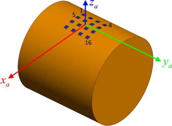
Figure 9: Antenna array on cylindrical PEC body.

Table 1: Emitter parameters

Emitter	r(km)	$\theta$(${}^{\circ }$)	$\varphi$(${}^{\circ }$)	Transmit Pow. (W)	G(dB)
Des.	100	35	50	don’t care
Undes. 1	100	35	140	0.1	20
Undes. 2	100	105	155	1	20
Undes. 3	100	165	105	2	20

Figure 10’s additional detail of element 11 includes the numbering (common to all 16 elements) of its two feed points (the physical points on the patch to which the ports are directly electrically connected by a probe feed). Each feed point corresponds to a nominally orthogonal linear polarization in the direction normal to the element’s copper patch. In [1] we configured each element for single-port operation (thus needing only one complex weight) by applying the same signal to both feed points but with an additional 90${}^{\circ }$ phase lag for feed point 2 with respect to feed point 1. This configuration achieved nominally RHC polarization in the direction normal to the element’s patch.

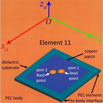
Figure 10: Detail of antenna element 11.

For this paper’s generalized algorithm, we assume the receiver/spatial-processor structure of Figure 8 and seek the 32 complex weights to maximize (90). To this end we first populate the parameters of the desired and undesired emitters’ antenna models of Figure 6 and Figure 7, respectively, using the technique of [16]. We then use a CES (FEKO’s method-of-moments (MoM) solver) to calculate the far-field vector electric-field data for each port of each antenna element with that port enabled and the other 31 ports disabled. We collect the far-field vector electric-field data at a constant slant range of 100 km for $0^{{}^{\circ }}\le \theta \le {180}^{{}^{\circ }}$ and $0^{{}^{\circ }}\le \varphi <{360}^{{}^{\circ }}$ in $5^{{}^{\circ }}$ increments each. To populate the parameters of the model of Figure 5 for all 32 ports, we process the electric-field data according to (24)–(28), assuming the phase center is at the center of the corresponding element’s copper patch.

Table 2 shows FEKO’s electric-field solution and the corresponding antenna-model parameters for the first element’s first port for $\theta ={35}^{{}^{\circ }}$ and $\varphi ={50}^{{}^{\circ }}$.

Table 2: MoM solution and corresponding antenna-model parameters for m = p = 1 at $\theta$ = ${35}^{{}^{\circ }}$ and $\varphi$ = ${50}^{{}^{\circ }}$

Re[Ẽ${}_{\mathrm{1}}$${}^{\mathrm{(}}$${}^a$${}^{\mathrm{,}\mathrm{1}\mathrm{,}}$${}^{\mathrm{1}}$${}^{\mathrm{)}}$($\theta$,$\varphi$)]	–1.5550709 $\times$ 10${}^{-5}$ V m${}^{-}$${}^1$
Im[Ẽ${}_{\mathrm{1}}$${}^{\mathrm{(}}$${}^a$${}^{\mathrm{,}\mathrm{1}\mathrm{,}}$${}^{\mathrm{1}}$${}^{\mathrm{)}}$($\theta$,$\varphi$)]	3.50444601 $\times$ 10${}^{-}$${}^6$ V m${}^{-1}$
E${}_{\mathrm{1}}$${}^{\mathrm{(}}$${}^a$${}^{\mathrm{,}\mathrm{1}\mathrm{,}}$${}^{\mathrm{1}}$${}^{\mathrm{)}}$($\theta$,$\varphi$)	1.59406930 $\times$ 10${}^{-5}$ V m${}^{-1}$
$\gamma$${}_1$${}^{(}$${}^a$${}^{,1,}$${}^1$${}^{)}$($\theta$,$\varphi$)	2.919939365 rad
K${}_{\mathrm{1}}$${}^{\mathrm{(}}$${}^a$${}^{\mathrm{,}\mathrm{1}\mathrm{,}}$${}^{\mathrm{1}}$${}^{\mathrm{)}}$($\theta$,$\varphi$)	0.00113871745
$\tau$${}_1$${}^{(}$${}^a$${}^{,1,}$${}^1$${}^{)}$($\theta$,$\varphi$)	1.89938530409 $\times$ 10${}^{-10}$ s
k${}_{\mathrm{1}}$${}^{\mathrm{(}}$${}^a$${}^{\mathrm{,}\mathrm{1}\mathrm{,}}$${}^{\mathrm{1}}$${}^{\mathrm{)}}$	525,505
Re[Ẽ${}_{\mathrm{2}}$${}^{\mathrm{(}}$${}^a$${}^{\mathrm{,}\mathrm{1}\mathrm{,}\mathrm{1}\mathrm{)}}$($\theta$,$\varphi$)]	2.03270802 $\times$ 10${}^{-5}$ V m${}^{-1}$
Im[Ẽ${}_{\mathrm{2}}$${}^{\mathrm{(}}$${}^a$${}^{\mathrm{,}\mathrm{1}\mathrm{,}\mathrm{1}\mathrm{)}}$($\theta$,$\varphi$)]	–6.2683354 $\times$ 10${}^{-}$${}^6$ V m${}^{-1}$
E${}_{\mathrm{2}}$${}^{\mathrm{(}}$${}^a$${}^{\mathrm{,}\mathrm{1}\mathrm{,}\mathrm{1}\mathrm{)}}$($\theta$,$\varphi$)	2.12716294 $\times$ 10${}^{-5}$ V m${}^{-1}$
$\gamma$${}_2$${}^{(}$${}^a$${}^{,1,1)}$($\theta$,$\varphi$)	–0.2991212046 rad
K${}_{\mathrm{2}}$${}^{\mathrm{(}}$${}^a$${}^{\mathrm{,}\mathrm{1}\mathrm{,}\mathrm{1}\mathrm{)}}$($\theta$,$\varphi$)	0.0015195309
$\tau$${}_2$${}^{(}$${}^a$${}^{,1,1)}$($\theta$,$\varphi$)	5.151403190 $\times$ 10${}^{-10}$ s
k${}_{\mathrm{2}}$${}^{\mathrm{(}}$${}^a$${}^{\mathrm{,}\mathrm{1}\mathrm{,}\mathrm{1}}$${}^{\mathrm{)}}$	525,505

Table 3 lists the complex weights calculated with (92) and (94). To find the optimally weighted array’s total and effective receive-gain patterns, we firstly exploit the principle of reciprocity by applying the calculated complex weights to the respective ports as source-signal amplitudes and phases. We then use FEKO’s MoM solver to numerically calculate the total and effective (RHC-polarization, in this case) transmit-gain patterns.

Table 3: Complex weights

m	p	Value
1	1	0.077819763793407 – j0.029465368993892
2	0.12459247349541 + j0.056703522041672
2	1	0.04516455849397 + j0.088872686331463
2	–0.065219319424497 + j0.12102226092079
3	1	–0.084334092382453 + j0.05080185997583
2	–0.080437225078455 –j0.03253844379338
4	1	–0.064700015503375 –j0.09520474257253
2	–0.006716174970139 –j0.09855765370402
5	1	0.07240921216198 +j0.128209559888171
2	–0.15646309053785 +j0.092759629157202
6	1	–0.1181600997625 +j0.0987977754199944
2	–0.12530905300321 –j0.158594127589902
7	1	0.121564402276342 –j0.100967272857737
2	0.129714464685709 –j0.137050242386695
8	1	0.086584951359559 –j0.138732803481413
2	0.17288811461883 +j0.089184429403536
9	1	–0.14794676203213 +j0.222500477675839
2	–0.18429998546202 –j0.104658615087023
10	1	–0.24105956227135 –j0.087952073329248
2	0.09175938725054 –j0.211979313185187
11	1	0.036227149294823 –j0.253494967774504
2	0.20696199056989 +j0.044332359948352
12	1	0.23987987902997 –j0.0066528888725053
2	0.003340598877023 +j0.21313132797126
13	1	–0.15316226330551 –j0.026851522912361
2	–0.036866990090258 –j0.13751921996212
14	1	0.0022933490913445 –j0.16987881222102
2	0.15162145119333 –j0.0696164846633674
15	1	0.160637367698868 –j0.026138400102631
2	0.056684020299592 +j0.15759987438645
16	1	0.040167786422328 +j0.17579356008101
2	–0.13038580760452 +j0.081501570656114

The annotated plots of Figure 11 and Figure 12 respectively show the achieved total-gain and effective-gain patterns. Clearly, the resulting gain patterns favor the desired emitter’s angular location with high total gain and nearly equal effective (i.e., RHC-polarization) gain, indicating very low polarization-mismatch loss due to an excellent match to the desired emitter’s polarization. In sharp contrast, however, the resulting gain patterns disfavor the undesired emitters’ angular locations with significantly lower total gains and strikingly lower RHC-polarization gains, indicating very high polarization-mismatch losses due to nearly perfect mismatches to the undesired emitters’ polarization. That is, in the directions of the undesired emitters, the optimally weighted array’s polarization states are nearly perfectly antipodal to the undesired emitters’ RHC polarization states [19]. Also, as we intuitively expect, the spatial-processing algorithm’s calculated weights result in the deepest effective null to counter the most powerful undesired emitter.

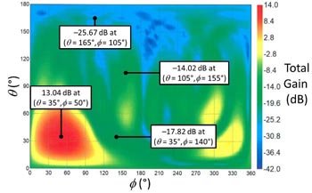
Figure 11: Total-gain pattern of optimally weighted array.

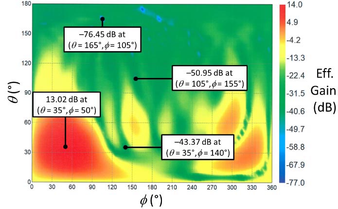
Figure 12: Effective-gain pattern of optimally weighted array.

Table 4 lists the achieved antenna gain and polarization characteristics corresponding to the desired and undesired emitters’ directions for three spatial-processing algorithms. Firstly, the traditional spatial-processing algorithm of [12] uses each individual element’s (total) receive directivity (as calculated with FEKO’s MoM solver) in the directions of all emitters due to the element itself, the cylindrical body, and the other elements. However, when calculating its sixteen complex weights, this first approach does not account for the apparent signal phase shifts (time delays) introduced within each individual element. Note that this first approach assumes each element is nominally RHC polarized (i.e., each element has a single port which drives both patch feed points with equal amplitude but with a 90${}^{\circ }$ phase lag applied between the element’s single port and its second feed point). Secondly, we repeat the results of the modern, improved algorithm of [1]. Like the traditional algorithm, the improved algorithm assumes single-port, nominally RHC-polarized elements. However, when calculating the sixteen complex weights, the improved algorithm does account for each individual element’s apparent internal attenuations and phase shifts using the high-fidelity antenna model of [15]. Thirdly, we report the results of this paper’s generalized algorithm in which we apply the thirty-two complex weights to their corresponding array ports (each connected directly to a patch feed point).

Table 4: Achieved antenna gain and polarization characteristics in emitter directions

Traditional	Improved	Generalized
Algorithm	Algorithm	Algorithm
Desired Emitter
G	12.65 dB	12.78 dB	13.04 dB
G${}_{e\mathit{}f\mathit{}f}$	12.63 dB	12.76 dB	13.02 dB
L${}_{p\mathit{}m\mathit{}m}$	0.02 dB	0.02 dB	0.02 dB
R	1.137	1.149	1.159
$\alpha$	63.53${}^{\circ }$	63.87${}^{\circ }$	19.53${}^{\circ }$
s	R	R	R
Undesired Emitter 1
G	–2.64 dB	–29.08 dB	–17.82 dB
G${}_{e\mathit{}f\mathit{}f}$	–2.72 dB	–43.24 dB	–43.37 dB
L${}_{p\mathit{}m\mathit{}m}$	0.09 dB	14.16 dB	25.56 dB
R	1.329	1.500	1.112
$\alpha$	175.84${}^{\circ }$	21.21${}^{\circ }$	74.61${}^{\circ }$
s	R	L	L
Undesired Emitter 2
G	–15.54 dB	–25.83 dB	–14.02 dB
G${}_{e\mathit{}f\mathit{}f}$	–18.85 dB	–49.54 dB	–50.95 dB
L${}_{p\mathit{}m\mathit{}m}$	3.30 dB	23.71 dB	39.94 dB
R	30.488	1.140	1.029
$\alpha$	143.22${}^{\circ }$	85.97${}^{\circ }$	88.28${}^{\circ }$
s	L	L	L
Undesired Emitter 3
G	–24.81 dB	–32.59 dB	–25.67 dB
G${}_{e\mathit{}f\mathit{}f}$	–30.32 dB	–65.61 dB	–76.45 dB
L${}_{p\mathit{}m\mathit{}m}$	5.52 dB	33.02 dB	50.79 dB
R	4.333	1.046	1.006
$\alpha$	30.03${}^{\circ }$	31.03${}^{\circ }$	118.56${}^{\circ }$
s	L	L	L

The results listed in Table 4 indicate the improved algorithm of [1] drastically outperforms the traditional algorithm in nullsteering. Specifically, the improved algorithm yielded much lower effective gain (the most important figure of merit highlighted in yellow in Table 4) in each undesired emitter’s direction. The improved algorithm also yielded modestly better beamforming as evidenced by its higher effective gain in the desired emitter’s direction. The improved algorithm’s performance advantage stems from complex weights calculated using high-fidelity quantitative data describing each element’s apparent internal attenuations and delays which account for that element’s inherent structure and the presence of the body and the other elements.

The results listed in Table 4 also indicate this paper’s generalized algorithm yields even better nullsteering and beamforming than the improved algorithm. The generalized algorithm’s performance advantage stems from the algorithm’s high-fidelity calculation of complex weights for both ports of each dual-polarization element. Note that the generalized algorithm produced typically modest performance advantages over the improved algorithm as compared to the conspicuous performance advantages the improved algorithm demonstrated over the traditional algorithm. The only exception to this was the significantly lower effective gain in the direction of undesired emitter 3–the interference source producing the highest spatial power density at the receive array’s location.

Interestingly, for this example scenario, the generalized spatial-processing algorithm achieved its lower effective gains via combinations of higher total gain and much higher polarization-mismatch loss as compared to the improved spatial-processing algorithm’s results. Note that the generalized algorithm’s performance improvements require more advanced antenna elements to transmit and/or receive two nominally orthogonal polarizations, additional CES computations to characterize the extra port models, more computations to obtain the optimal complex weights, and a more complex receiver/spatial processor to modify and combine the additional signals.

V. CONCLUSION

This paper generalized a recently improved spatial-processing algorithm for arrays of potentially diverse antenna elements arbitrarily arranged on a body of arbitrary shape and material composition. Whereas the improved algorithm applied exclusively to arrays of single-port elements, the generalized algorithm supports arrays of dual-polarization antenna elements. Unlike traditional spatial-processing algorithms, the generalized algorithm requires high-fidelity far-field gain and polarization data in the directions of the desired and undesired communication nodes for both ports of each array element. Only a CES or sophisticated testing can provide such data since each element’s data must account for the presence of the body and the other antenna elements. The generalized algorithm also requires the total gain and polarization characteristics of each desired and undesired communication node’s antenna in the direction of the antenna array. After appropriate processing this information populates the parameters of recently developed high-fidelity antenna models (both transmit and receive modes). The generalized algorithm uses the populated antenna models to obtain a highly detailed expression for SIR which is mathematically compatible with the traditional technique for calculating the optimal complex weights. In an illustrative practical example simulated with high fidelity via a CES, the generalized spatial-processing algorithm outperformed both the improved algorithm and the traditional algorithm.

This paper’s investigation and development suggest several potential avenues for additional, related work. Firstly, space-time adaptive processing [12, 13, 14] may exhibit improved performance after a straightforward integration of this paper’s high-fidelity spatial-processing technique. Secondly, in Section IV the generalized algorithm achieved its exceptional performance using double-precision computations to calculate complex weights having about fifteen significant digits in both their real and imaginary parts. However, some practical (e.g., legacy) systems can only effect much coarser control of signal amplitude and phase. Thus, an investigation of the generalized algorithm’s performance under such limitations could help assess the breadth of the algorithm’s practical applicability. Thirdly, adapting this paper’s algorithm to arrays comprising arbitrary combinations of single-polarization and dual-polarization elements represents a further yet straightforward generalization. Fourthly, one may adapt this paper’s generalized algorithm to use antenna-element models with orthogonally circularly polarized components as described in [20, 21] rather than orthogonally linearly polarized components. Fifthly, the gain and polarization data describing the undesired emitters may not be available. In such cases we may still use the high-fidelity representation of (64) and (80), assuming the desired emitter’s location and antenna properties are available. However, we must approximate (91) with sample-mean techniques [12]. A performance comparison of this suboptimal but practical technique with this paper’s optimal but potentially impractical technique might characterize the degradation in results. Finally, Section IV’s results suggest the generalized algorithm may rely on high polarization-mismatch losses (as opposed to low total gains) to achieve its exceptional effective null depths. Even a modest change in an undesired emitter’s antenna polarization may yield significantly greater RFI penetration of the receiver/spatial processor. Some suitable algorithm modifications might produce lower total gains in the directions of the undesired emitters, perhaps at the expense of lower polarization-mismatch losses. Such a modified spatial-processing algorithm may increase the receive array’s overall robustness to any variations in the undesired emitters’ polarization states by making the algorithm less reliant on closely matching the array to polarization states antipodal to those of the undesired emitters.

REFERENCES

[1] J. Spitzmiller, “Improved spatial processing through high-fidelity antenna modeling,” IEEE/ION Position, Location, and Navigation Symposium, Portland, OR, April 2020.

[2] W. Stutzman and G. Thiele, Antenna Theory and Design, 3rd ed., John Wiley & Sons, Hoboken, 2013.

[3] C. Pang, P. Hoogeboom, F. Le Chevalier, H. Russchenberg, J. Dong, T. Wang, and X. Wang, “Dual-polarized planar phased array analysis for meteorological applications,” International Journal of Antennas and Propagation, 2015.

[4] Z. Chen, T. Li, D. Peng, and K. Du, “Two-dimensional beampattern synthesis for polarized smart antenna array and its sparse array optimization,” International Journal of Antennas and Propagation, 2020.

[5] R. Fante, “Principles of adaptive space-time-polarization cancellation of broadband interference,” MITRE Corporation, 2004.

[6] H. Wang, L. Yang, Y. Yang, and H. Zhang, “Anti-jamming of Beidou navigation based on polarization sensitive array,” Int. Applied Comp. Electromagnetics Society (ACES) Symp., Suzhou, China, August 2017.

[7] I. D. Olin, “Polarization characteristics of coherent waves,” Naval Research Laboratory publications, NRL/FR/5317-12-10,210, 2012.

[8] C. Liu, Z. Ding, and X. Liu, “Pattern synthesis for conformal arrays with dual polarized antenna elements,” 7th Int. Congress on Image and Signal Proc., Dalian, China, pp. 968-973, October 2014.

[9] H. Li, T. Wang, and X. Huang, “Joint adaptive AoA and polarization estimation using hybrid dual-polarization antenna arrays,” IEEE Access, vol. 7, 2019.

[10] M. Golbon-Haghighi, M. Mirmozafari, H. Saeidi-Manesh, and G. Zhang, “Design of a cylindrical crossed dipole phased array antenna for weather surveillance radars,” IEEE Open Journal of Antennas and Propagation, vol. 2, pp. 402-411,2021.

[11] E. McMilin, Y. Chen, D. De Lorenzo, D. Akos, T. Walter, T. Lee, and P. Enge, “Single antenna, dual use,” Inside GNSS, September/October 2015, pp. 40-53, 2015.

[12] M. Budge, Jr. and S. German, Basic Radar Analysis, 2nd ed., Artech House, Boston, 2020.

[13] J. Guerci, Space-Time Adaptive Processing, 2nd ed., Artech House, Boston, 2015.

[14] M. Richards, Fundamentals of Radar Signal Processing, 2nd ed., McGraw-Hill, New York, 2014.

[15] J. Spitzmiller, “Antenna model using ideal passive RF components,” IEEE SoutheastCon, Raleigh, NC, March 2020.

[16] J. Spitzmiller, “Antenna model from total gain and polarization characteristics,” IEEE SoutheastCon, Raleigh, NC, March 2020.

[17] I. Cumming and F. Wong, Digital Processing of Synthetic Aperture Radar Data, Artech House, Boston, 2005.

[18] P. Peebles, Jr., Communication System Principles, Addison-Wesley, Reading, 1976.

[19] J. Kraus, Antennas, 2nd ed., McGraw-Hill, New York, 1988.

[20] J. Spitzmiller, “Antenna model using ideal passive RF components and circularly polarized antenna elements,” IEEE SoutheastCon, Atlanta, GA, March 2021.

[21] J. Spitzmiller, “Antenna model using circularly polarized elements from total gain and polarization characteristics,” IEEE SoutheastCon, Atlanta, GA, March 2021.

BIOGRAPHIES

John Spitzmiller has worked for Parsons (formerly Cobham Analytic Solutions and SPARTA, Inc.) in Huntsville, Alabama since 2006. He has served as Chief Engineer of Offensive Missile Programs since 2011. In this position he has worked on a wide variety of efforts involving analysis, modeling, simulation, and assessment of radar, RF-navigation, RF-telemetry, and electronic-warfare systems. Parsons named him a Fellow in 2018. From 1999 to 2006, he served as an electronics engineer in the Scientific and Technical Modeling and Simulation Branch of the Defense Intelligence Agency’s Missile and Space Intelligence Center on Redstone Arsenal, Alabama. From 1995 to 1999, he worked in the Sensor Systems and Technologies Department at Dynetics, Inc. in Huntsville, Alabama. A 1994 Goldwater Scholar, he graduated summa cum laude with a B.S. in electrical engineering from the University of Missouri at Rolla in 1995. He subsequently earned an M.S.E. and Ph.D. in electrical engineering from the University of Alabama in Huntsville. His current research interests include advanced techniques for signal, image, and spatial processing and linear and nonlinear state estimation.

Sanyi Choi is a senior engineer at Parsons Government Services, where she has been employed since 2018. She is responsible for performing radar system analysis, modeling, and simulation. She has primarily supported the Defense Intelligence Agency/Missile and Space Intelligence Center (DIA/MSIC) with advanced signal processing methodologies and Synthetic Aperture Imaging. From 2010 to 2018 she was with Northrop Grumman Corp. in Huntsville, Alabama where she worked in Enhanced Command and Control Battle Management and Communications (EC2BMC) activities in support of the Missile Defense Agency (MDA) as a system engineer supporting on the development of advanced discrimination algorithm. She earned a B.S.E. and M.S.E. in electrical engineering from the University of Alabama in Huntsville.

ACES JOURNAL, Vol. 37, No. 1, 19–33.
doi: 10.13052/2022.ACES.J.370103
© 2021 River Publishers