Reduction of Random Variables in EMC Uncertainty Simulation Model

Jinjun Bai¹, Yixuan Wan¹, Ming Li², Gang Zhang³, and Xin He³

¹Department of Electrical Engineering, Dalian Maritime University, Dalian, 116026, China
baijinjun@dlmu.edu.cn, wanyixuan90@163.com

²Aviation Industry Corporation of China (AVIC), AVIC Aero Polytechnol Estab, Beijing 100028, Peoples R China
liming_mse_buaa@163.com

³Harbin Inst Technol, Sch Elect Engn & Automat, Harbin Institute of Technology,Harbin 150001, Peoples R China
zhang_hit@hit.edu.cn,19s106116@stu.hit.edu.cn

Submitted On: December 13, 2021; Accepted On: August 13, 2022

Abstract

To improve the reliability of simulation results, uncertainty analysis methods were developed in the Electromagnetic Compatibility (EMC) field. Random variables are used to describe random events. The more random variables you have, the less efficient the simulation is. Therefore, many high-accuracy methods have the problem of dimensional disaster, which means the calculation efficiency decreases exponentially with the increase of the number of random variables. A random variable reduction strategy based on sensitivity analysis method is proposed in this paper, so as to improve the computational efficiency of the global uncertainty analysis method.

Index Terms: dimensional disaster, electromagnetic compatibility, random variable, sensitivity analysis method, uncertainty analysis method.

I. INTRODUCTION

To describe random events and unknown parameters in a practical engineering environment, the uncertainty analysis method is becoming popular in the EMC field. The random variable model is used to describe the actual uncertainty factors instead of the deterministic values.

Uncertainty analysis methods can be divided into two categories. In one class, some of the methods need to change the original solver, such as the Perturbation Method [1], the Stochastic Galerkin Method [2, 3], and the Stochastic Testing Method [4]. In general, to describe complex electromagnetic compatibility problems in practical engineering environment, the finite element analysis method is used to construct model parameters, and then commercial simulation software is needed. The software is not open source, and cannot change the original internal solver. Therefore, this class of uncertainty analysis method is not competitive in the EMC field.

Another class of methods does not need to change solver, represented by the Monte Carlo Method [5, 6], the Stochastic Reduced Order Models [7], the Moment Method [8], and the Stochastic Collocation Method (SCM) [9, 10]. They are suitable for different EMC simulation situations. The Monte Carlo Method has high accuracy and low computational efficiency. It is suitable for uncertainty analysis with a short simulation time. For complex problems, it will lose competitiveness because of its low computational efficiency. The advantage of the Stochastic Reduced Order Models and the Moment Method is high computational efficiency. However, in most cases, their accuracy is not as good as other methods. The Stochastic Reduced Order Models have low accuracy due to the lack of an appropriate convergence criterion. The Moment Method assumes that the simulation input and simulation output are linear, which leads to its low accuracy. The advantages of the SCM combine computational efficiency and accuracy, but it is trapped in the problem of dimension disaster. This means that the number of collocation points increases exponentially with the number of random variables. Many scholars have improved the SCM to alleviate the dimension disaster problem slightly [11]. To completely solve this problem, it is still necessary to fundamentally reduce the number of randomvariables.

Based on the thoughts of the Moment Method, this paper proposes a fast sensitivity calculation method, which directly transfers the random variables with low sensitivity to the average values. It can be predicted that the longer single EMC simulation time, the more significant the improvement of computing efficiency will be.

II. SENSITIVITY ANALYSIS BASED ON THE RICHARDSON EXTRAPOLATION METHOD

When the EMC simulation model is in the form of random variables, the output will present uncertainty. The contribution of each random variable to the uncertainty of simulation output is different. If the contribution can be expressed quantitatively, the random variable with a smaller contribution can be replaced by its average value, so as to achieve the reduction of the random variables.

The contribution can be described by means of sensitivity analysis, while all uncertainty analysis methods can realize sensitivity analysis by calculating standard deviation. It should be noted that the sensitivity analysis method proposed in this paper is a pre-processing step of the uncertainty analysis method, so its solving speed must be far better than that of the uncertainty analysis method, otherwise, the reduction of random variables will be meaningless.

In the Moment Method, the sensitivity analysis of each random variable is used to estimate variance values. The sensitivity calculation process is shown below:

$S(i)={\displaystyle \frac{d{y}_{\xi }}{d{\xi }_i}}$	(1)
$={\displaystyle \frac{U_{EMC}(\overline{{\xi }_1},\mathrm{\cdots },\overline{{\xi }_i}+{\delta }_i,\mathrm{\cdots },\overline{{\xi }_n})}{{\delta }_i}}$
$-{\displaystyle \frac{U_{EMC}(\overline{{\xi }_1},\mathrm{\cdots },\overline{{\xi }_i},\mathrm{\cdots },\overline{{\xi }_n})}{{\delta }_i}}.$

Among them, $\overline{{\xi }_i}$ represents the mean value of random variable ${\xi }_i$, and $U_{EMC}(\overline{{\xi }_1},\mathrm{\cdots },\overline{{\xi }_i},\mathrm{\cdots },\overline{{\xi }_n})$ represents the EMC simulation result at a certain point $(\overline{{\xi }_1},\overline{{\xi }_i},\mathrm{\cdots },\overline{{\xi }_n})$. ${\delta }_i$ is a small perturbation, and S(i) is the sensitivity analysis result corresponding to random variable ${\xi }_i$. Its principle is to transform the differential formula into a difference formula.

The selection of perturbation is based on the uniform distribution. Suppose that the uncertainty parameter is $k\left({\xi }_i\right)=A+B\times {\xi }_i$, where ${\xi }_i$ is the uniform distribution variable of the interval [-1,1] . In this case, the perturbation is ${\delta }_i={\displaystyle \frac{B}{A}}$. However, not all uncertain parameters are in the form of uniform distribution, thus it is necessary to convert them into an equivalent uniform distribution. It is assumed that the mean value of uncertain parameters is $k_M$, the variance of that is $k_{\sigma }$. The equation can be converted as follow:

$$\{\begin{array}{c}\hfill k_M=A\hfill \\ \hfill k_{\sigma }=\frac{1}{3}{B}^2.\hfill \end{array}$$

(2)

Therefore, the perturbation is ${\delta }_i={\displaystyle \frac{\sqrt{3k_{\sigma }}}{k_M}}$.

Reference [8] mentions that the Moment Method does not achieve very good accuracy, which is mainly due to the following two reasons. On one hand, the Moment Method assumes that the input and output are in a linear relationship, which leads to calculation error of sensitivity S(i) in formula (1). On the other hand, this formula only considers the disturbance quantity when it is greater than the average value, the sensitivity estimated does not represent the whole situation at this time. To solve this nonlinear problem, the Richardson extrapolation method is proposed to improve the different processes in formula (1), as shown below:

$I{S}_{pos}(i)={\displaystyle \frac{d{y}_{\xi }}{d{\xi }_i}}$	(3)
$=2\times {\displaystyle \frac{U_{EMC}(\overline{{\xi }_1},\mathrm{\cdots },\overline{{\xi }_i}+{\displaystyle \frac{{\delta }_i}{2}},\mathrm{\cdots },\overline{{\xi }_n})}{{\displaystyle \frac{{\delta }_i}{2}}}}$
$-2\times {\displaystyle \frac{U_{EMC}(\overline{{\xi }_1},\mathrm{\cdots },\overline{{\xi }_i},\mathrm{\cdots },\overline{{\xi }_n})}{{\displaystyle \frac{{\delta }_i}{2}}}}$
$-{\displaystyle \frac{U_{EMC}(\overline{{\xi }_1},\mathrm{\cdots },\overline{{\xi }_i}+{\delta }_i,\mathrm{\cdots },\overline{{\xi }_n})}{{\delta }_i}}$
$+{\displaystyle \frac{U_{EMC}(\overline{{\xi }_1},\mathrm{\cdots },\overline{{\xi }_i},\mathrm{\cdots },\overline{{\xi }_n})}{{\delta }_i}},$

$I{S}_{neg}(i)={\displaystyle \frac{d{y}_{\xi }}{d{\xi }_i}}$	(4)
$=2\times {\displaystyle \frac{U_{EMC}(\overline{{\xi }_1},\mathrm{\cdots },\overline{{\xi }_i}-{\displaystyle \frac{{\delta }_i}{2}},\mathrm{\cdots },\overline{{\xi }_n})}{{\displaystyle \frac{{\delta }_i}{2}}}}$
$-2\times {\displaystyle \frac{U_{EMC}(\overline{{\xi }_1},\mathrm{\cdots },\overline{{\xi }_i},\mathrm{\cdots },\overline{{\xi }_n})}{{\displaystyle \frac{{\delta }_i}{2}}}}$
$-{\displaystyle \frac{U_{EMC}(\overline{{\xi }_1},\mathrm{\cdots },\overline{{\xi }_i}-{\delta }_i,\mathrm{\cdots },\overline{{\xi }_n})}{{\delta }_i}}$
$+{\displaystyle \frac{U_{EMC}(\overline{{\xi }_1},\mathrm{\cdots },\overline{{\xi }_i},\mathrm{\cdots },\overline{{\xi }_n})}{{\delta }_i}}.$

The proposed algorithm considers both sides, that is, there are positive sensitivity $I{S}_{pos}(i)$ and negative sensitivity $I{S}_{neg}(i)$. The mathematical derivation of the Richardson extrapolation method is as follows. The complete calculation formula corresponding to formula (1) is:

${\displaystyle \frac{d{y}_{\xi }}{d{\xi }_i}}={\displaystyle \frac{U_{EMC}(\overline{{\xi }_1},\mathrm{\cdots },\overline{{\xi }_i}+{\delta }_i,\mathrm{\cdots },\overline{{\xi }_n})}{{\delta }_i}}$	(5)
$-{\displaystyle \frac{U_{EMC}(\overline{{\xi }_1},\mathrm{\cdots },\overline{{\xi }_i},\mathrm{\cdots },\overline{{\xi }_n})}{{\delta }_i}}-{\displaystyle \frac{{\delta }_i}{2}}\times y_{\xi }^{\prime \prime }+o\left({\delta }_i\right).$

When using formula (1) to calculate sensitivity, the error is ${\displaystyle \frac{{\delta }_i}{2}}\times y_{\xi }^{\prime \prime }.$

By changing the perturbation in formula (5) into ${\displaystyle \frac{{\delta }_i}{2}}$, formula (6) can be obtained:

${\displaystyle \frac{d{y}_{\xi }}{d{\xi }_i}}={\displaystyle \frac{U_{EMC}(\overline{{\xi }_1},\mathrm{\cdots },\overline{{\xi }_i}+{\displaystyle \frac{{\delta }_i}{2}},\mathrm{\cdots },\overline{{\xi }_n})}{{\displaystyle \frac{{\delta }_i}{2}}}}$	(6)
$-{\displaystyle \frac{U_{EMC}(\overline{{\xi }_1},\mathrm{\cdots },\overline{{\xi }_i},\mathrm{\cdots },\overline{{\xi }_n})}{{\displaystyle \frac{{\delta }_i}{2}}}}-{\displaystyle \frac{{\delta }_i}{4}}\times y_{\xi }^{\prime \prime }+o\left({\delta }_i\right).$

Multiplying formula (6) by 2 and subtracting formula (5), formula (7) is presented:

${\displaystyle \frac{d{y}_{\xi }}{d{\xi }_i}}=2\times {\displaystyle \frac{U_{EMC}(\overline{{\xi }_1},\mathrm{\cdots },\overline{{\xi }_i}+{\displaystyle \frac{{\delta }_i}{2}},\mathrm{\cdots },\overline{{\xi }_n})}{{\displaystyle \frac{{\delta }_i}{2}}}}$	(7)
$-2\times {\displaystyle \frac{U_{EMC}(\overline{{\xi }_1},\mathrm{\cdots },\overline{{\xi }_i},\mathrm{\cdots },\overline{{\xi }_n})}{{\displaystyle \frac{{\delta }_i}{2}}}}$
$-{\displaystyle \frac{U_{EMC}(\overline{{\xi }_1},\mathrm{\cdots },\overline{{\xi }_i}+{\delta }_i,\mathrm{\cdots },\overline{{\xi }_n})}{{\delta }_i}}$
$+{\displaystyle \frac{U_{EMC}(\overline{{\xi }_1},\mathrm{\cdots },\overline{{\xi }_i},\mathrm{\cdots },\overline{{\xi }_n})}{{\delta }_i}}+o\left({\delta }_i\right).$

By means of approximation, formula (3) results. Similarly, negative sensitivity shown in formula (4) can also be derived. Obviously, the approximate error is $o({\delta }_i)$, which is better than ${\displaystyle \frac{{\delta }_i}{2}}\times y_{\xi }^{\prime \prime }$ in formula (5).

A comprehensive index of both sides can be obtained by adding absolute values directly.

$$IS(i)=\left|I{S}_{pos}(i)\right|+\left|I{S}_{neg}(i)\right|.$$

(8)

The contribution of each random variable is represented by the percentage as follow:

$$P(i)=\frac{IS(i)}{\sum _{i=1}^{N}IS(i)}.$$

(9)

III. ALGORITHM VALIDATION

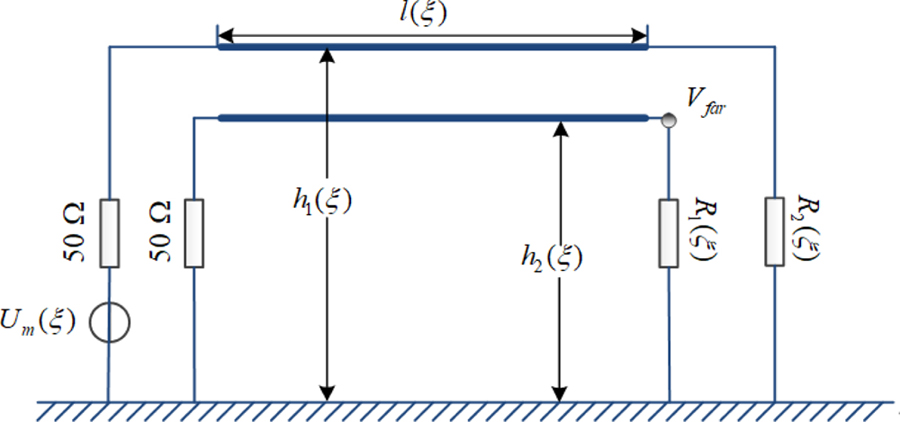
This section presents a benchmark calculating example in [10] to verify the accuracy of random variable reduction algorithm. It is a crosstalk simulation example with 6 uncertain parameters shown in Fig. 1. There is crosstalk source voltage $U_m(\xi )$, the height of two parallel cables $h_1(\xi )$ and $h_2(\xi )$, length of parallel cables $l(\xi )$, resistance value at load side $R_1(\xi )$ and $R_2(\xi )$.

$$U_m(\xi )=1.05+0.05\times {\xi }_1\mathrm{V},$$

(10)

$$h_1(\xi )=0.04\times \left(1.1+0.1\times {\xi }_2\right)\mathrm{m},$$

(11)

$$h_2(\xi )=0.03\times \left(1.15+0.15\times {\xi }_3\right)\mathrm{m},$$

(12)

$$l(\xi )=1.1+0.1\times {\xi }_4\mathrm{m},$$

(13)

$$R_1(\xi )=50\times \left(1.05+0.05\times {\xi }_5\right)\mathrm{\Omega },$$

(14)

$$R_2(\xi )=50\times \left(1.04+0.04\times {\xi }_6\right)\mathrm{\Omega }.$$

(15)

Among them,${\xi }_1$, ${\xi }_2$, ${\xi }_3$, ${\xi }_4$, ${\xi }_5$ and ${\xi }_6$ are all uniform distribution random variables in the interval [-1,1]. The horizontal distance between the two cables is 0.05m, and the frequency of crosstalk results is in 50MHz. The other detailed information of the model is completely consistent with reference [10].

Fig. 1: Benchmark calculating example in [10].

Table 1: Sensitivity analysis results of random variables

Variable	Sensitivity
${\xi }_1$	22$\%$
${\xi }_2$	16.9$\%$
${\xi }_3$	24.3$\%$
${\xi }_4$	35.1$\%$
${\xi }_5$	1$\%$
${\xi }_6$	0.7$\%$

Table 1 shows the sensitivity calculation results of the random variables. It can be seen that the sum weight of the random variables ${\xi }_5$ and ${\xi }_6$ is only 1.7$\%$, thus the average values can be adopted to replace them, as shown below.

$$R_1({\xi }_5=0)=50\times 1.05=52.5\mathrm{\Omega },$$

(16)

$$R_2({\xi }_6=0)=50\times 1.04=52\mathrm{\Omega }.$$

(17)

In this case, there are only four random variables left in the simplified EMC model.

Taking the SCM as an example, the uncertainty analysis results of voltage crosstalk in load side are calculated in both original model and simplified model respectively. According to the SCM, uniform distribution random variable in the interval [-1,1] is corresponding to the Legende orthogonal polynomial. If the probability density function is arbitrary, the chaotic polynomial form can be obtained by the three-term polynomial recursive formula in the Stieltjes Procedure. For details, please refer to literature [12].

Zero points of the 7th-order Legendre orthogonal polynomial are considered as the collocation points, they are shown as follows.

$P_{{\xi }_i}=\{0.9491,0.7415,0.4058,0,$	(18)
$-0.4058,-0.7415,-0.9491\}.$

In multiple random variables situation, the selection of collocation points takes the form of tensor product:

$$P_{{\xi }_i}\otimes P_{{\xi }_i}\otimes P_{{\xi }_i}\otimes P_{{\xi }_i}\otimes P_{{\xi }_i}\otimes P_{{\xi }_i}.$$

(19)

Multivariate Lagrange interpolation at the collocation points is implemented, the result in the form of random variables polynomial will be obtained.Through statistical sampling, the final uncertainty analysis results can be got, such as expectation, standard deviation and probability density curve.

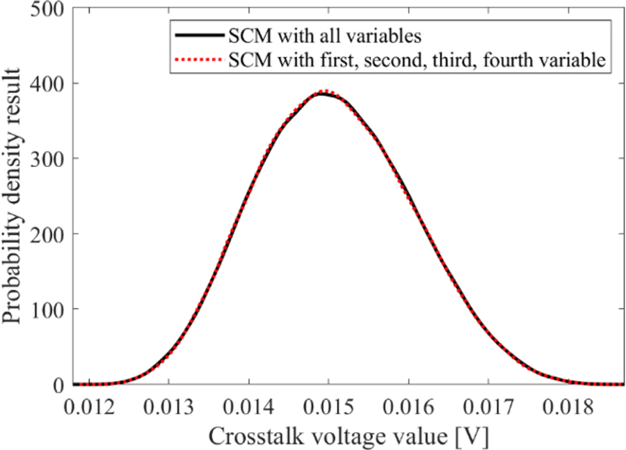
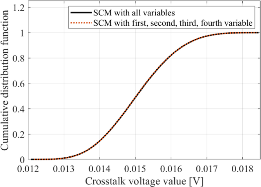
Figures 2 and 3 show the Probability Distribution Function (PDF) results and the Cumulative Distribution Function (CDF) results of crosstalk voltage values respectively. The results of 4-variables model and original model variables model are given at the same time. It is clearly seen that two curves are almost exactly the same in both Figs. 2 and 3, and it means that the reduction has no impact on accuracy. For quantitative comparison, the mean value calculated by original model is $0.01506\mathrm{V}$, and the standard deviation is $9.8058\times {10}^{-4}\mathrm{V}$. For 4-variables model, the mean value is $0.01506\mathrm{V}$ and the standard deviation is $9.7870\times {10}^{-4}\mathrm{V}$.

The Mean Equivalent Area Method (MEAM) is a validity evaluation method of uncertainty analysis results. The MEAM can evaluate the accuracy of simulation results by quantifying the similarity between simulation results and standard data. When the MEAM value of the simulation result is better than 0.95, its accuracy is considered “Excellent” [13]. For random variable reduction problem in this paper, the uncertainty analysis results of the original model are taken as the standard data, and the uncertainty analysis results of 4-variables model must be at the level of “Excellent”, so that the reduction is meaningful. In Figs. 2 and 3, the MEAM value of 4-variables model is 0.9981, which proves that the effect of reduction is good.

Fig. 2: PDF results of 4-variables model.

Fig. 3: CDF results of 4-variables model.

According to the generalized polynomial chaos theory [4], the original model requires the number of deterministic simulations is $7^6=117649$. As a comparison, the number of pre-processing simulations in 4-variables model is $4\times 6+1=25$, that of deterministic simulations is $7^4=2401$ Thus, in 4-variables model, a total of 2426 deterministic simulations are required. It means that the calculation amount of 4-variables model is only 2$\%$ of that of the original model. It is worth noting that the longer the single simulation time, the better the improvement of computational efficiency.

In summary, by comparing the required single simulation times, it is verified that the proposed reduction method in this paper improves the efficiency of the uncertainty analysis method. The validity of the reduction method is verified by comparing the expected value, standard deviation and MEAM value. Thus, it is proved that the reduction method can alleviate the dimension disaster of the SCM to some extent.

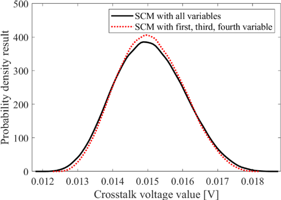
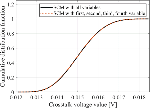
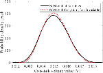
Fig. 4: PDF results of the model with ${\xi }_1$, ${\xi }_3$ and ${\xi }_4$.

Fig. 5: CDF results of the model with ${\xi }_1$, ${\xi }_3$ and ${\xi }_4$.

IV. DISCUSSION OF THE WEIGHT THRESHOLD

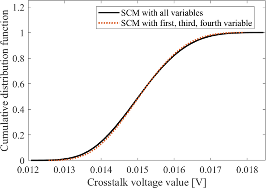
In Table 1, the percentage of ${\xi }_5$ and ${\xi }_6$ is small, so they can obviously be reduced. The effectiveness of reduction has been proved in Section III. If another random variable is reduced too, the computational efficiency will inevitably increase, but with the risk of accuracy decline. In this section, the weight threshold of percentage sum of retained random variables is quantitatively determined. As shown in Table 1, the percentage of ${\xi }_1$ and ${\xi }_2$ is the next smallest, two new simplified models are proposed. One is with the random variables ${\xi }_1$, ${\xi }_3$ and ${\xi }_4$. The other is with ${\xi }_2$, ${\xi }_3$ and ${\xi }_4$.

Figures 4 and 5 show PDF results and CDF results under random variables ${\xi }_1$, ${\xi }_3$ and ${\xi }_4$. The mean value of the result is $0.01507\mathrm{V}$, and the standard deviation of that is $9.2107\times {10}^{-4}\mathrm{V}$. The MEAM value is 0.9393, which is less than 0.95, but still in the acceptable range.

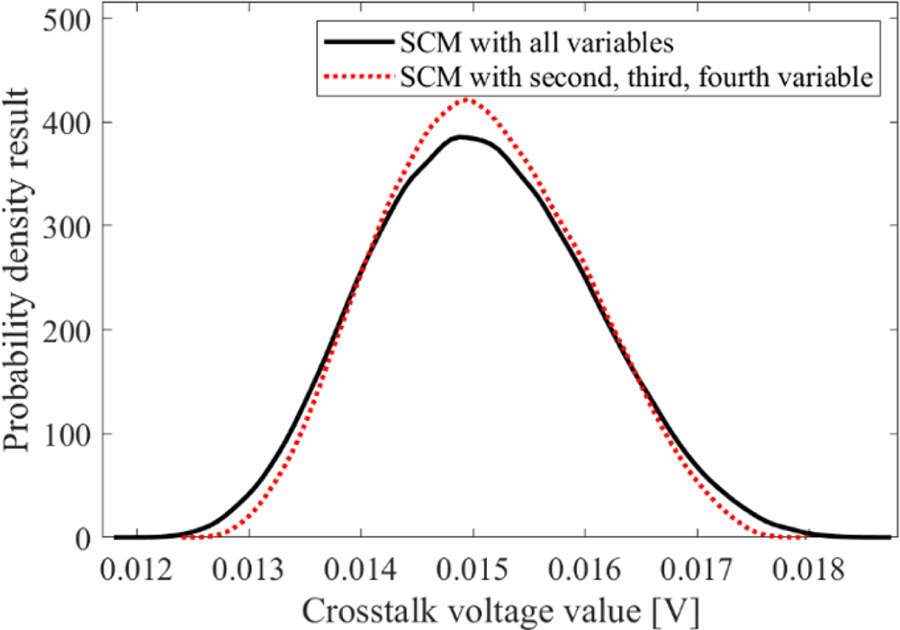
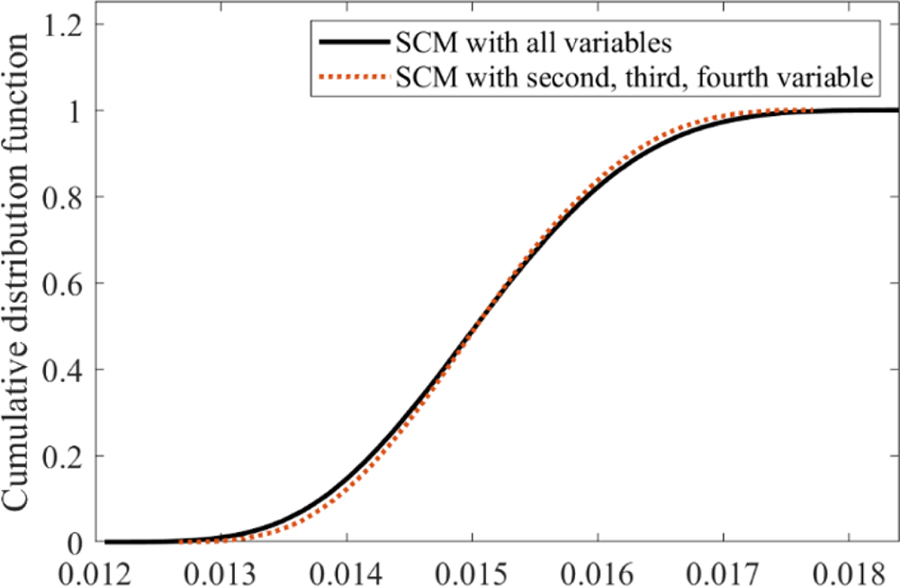
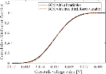
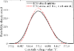
Figures 6 and 7 show PDF results and CDF results in random variables ${\xi }_2$, ${\xi }_3$ and ${\xi }_4$. The mean value of this model is $0.01507\mathrm{V}$, and the standard deviation is $8.8981\times {10}^{-4}\mathrm{V}$. The MEAM value is 0.9074, which has a gap of 0.95. In this case, the error of reduction is identified as large, so it is not acceptable.

Fig. 6: PDF results of the model with ${\xi }_2$, ${\xi }_3$ and ${\xi }_4$.

Fig. 7: CDF results of the model with ${\xi }_2$, ${\xi }_3$ and ${\xi }_4$.

After quantitative comparison of these two simplified models, the former one is barely acceptable, while the latter one is unacceptable. The weight threshold of them is 22$\%$ + 24.3$\%$ + 35.1$\%$ = 81.4$\%$ and 16.9$\%$ + 24.3$\%$ + 35.1$\%$ = 76.3$\%$. It can be seen that when the weight threshold is below 85$\%$, the uncertainty analysis results of the reduction model are not satisfactory. To ensure, it is better to set the weight threshold within the range of 90$\%$ to 95$\%$ in practical application, so as to ensure that the MEAM value can be maintained above 0.95, in an “Excellent” level.

V. CONCLUSION

Based on the Richardson extrapolation method, a sensitivity analysis method to evaluate the contribution of random variables is proposed to improve the EMC uncertainty simulation computational efficiency. The effectiveness of the proposed reduction method is verified by using a benchmark simulation example. On the premise of maintaining the original accuracy, the proposed method greatly improves the computational efficiency of the SCM, and the time required is only 2$\%$ of the previous time. It is proved that the reduction strategy can alleviate the dimension disaster problem of the SCM to a certain extent. Finally, through quantitative calculation by using the MEAM, it is determined that from 90$\%$ to 95$\%$ is a reasonable selection range of weight threshold.

REFERENCES

[1] Y. Zhang, C. Liao, R. Huan, Y. Shang, and H. Zhou, “Analysis of nonuniform transmission lines with a perturbation technique in time domain,” IEEE Transactions on Electromagnetic Compatibility, vol. 62, no. 2, pp. 542-548, 2020.

[2] P. Manfredi, D. Ginste, I. Stievano, D. De Zutter, and F. Canavero, “Stochastic transmission line analysis via polynomial chaos methods: An overview,” IEEE Electromagnetic Compatibility Magazine, vol. 6, no. 3, pp. 77-84, 2017.

[3] P. Manfredi, D. Vande. Ginste, D. De Zutter, and F. G. Canavero, “Generalized decoupled polynomial chaos for nonlinear circuits with many random parameters,” IEEE Microwave & Wireless Components Letters, vol. 25, no. 8, pp. 505-507, 2015.

[4] Z. Zhang, T. A. EI-Moselhy, I. M. Elfadel, and L. Daniel, “Stochastic testing method for transistor-level uncertainty quantification based on generalized polynomial chaos,” IEEE Transactions on Computer-Aided Design of Integrated Circuits and Systems, vol. 32, no. 10, pp. 1533-1545, 2013.

[5] S. A. Pignari, G. Spadacini, and F. Grassi, “Modeling field-to-wire coupling in random bundles of wires,” IEEE Electromagnetic Compatibility Magazine, vol. 6, no. 3, pp. 85-90, 2017.

[6] H. Xie, J. F. Dawson, J. Yan, A. C. Marvin, and M. P. Robinson, “Numerical and analytical analysis of stochastic electromagnetic fields coupling to a printed circuit board trace,” IEEE Transactions on Electromagnetic Compatibility, vol. 62, no. 4, pp. 1128-1135, 2020.

[7] Z. Fei, Y. Huang, J. Zhou, and Q. Xu, “Uncertainty quantification of crosstalk using stochastic reduced order models,” IEEE Transactions on Electromagnetic Compatibility, vol. 59, no. 1, pp. 228-239, 2016.

[8] R. S. Edwards, A. C. Marvin, and S. J. Porter, “Uncertainty analyses in the finite difference time domain method,” IEEE Transactions on Electromagnetic Compatibility, vol. 52, no. 1, pp. 155-163, 2010.

[9] T. Wang, Y. Gao. L. Gao, C. Liu, J. X. Wang, and Z. Y. An, “Statistical analysis of crosstalk for automotive wiring harness via the polynomial chaos method,” Journal of the Balkan Tribological Association, vol. 22, no. 2, pp. 1503-1517, 2016.

[10] J. Bai, G. Zhang, D. Wang, A. P. Duffy, and L.Wang, “Performance comparison of the sgm and the scm in emc simulation,” IEEE Transactions on Electromagnetic Compatibility, vol. 58, no. 6, pp. 1739-1746, Apr. 2016.

[11] J. Bai, G. Zhang, A. P. Duffy, and L. Wang, “Dimension-reduced sparse grid strategy for a stochastic collocation method in emc software,” IEEE Transactions on Electromagnetic Compatibility, vol. 60, no. 1, pp. 218-224, 2018.

[12] D. Xiu, E. Karniadakis, and George, “The wiener-askey polynomial chaos for stochastic differential equations,” SIAM Journal on Scientific Computing, vol. 24, no. 2, pp. 619-644, 2002.

[13] J. Bai, L. Wang, D. Wang, A. P. Duffy, and G. Zhang, “Validity evaluation of the uncertain emc simulation results,” IEEE Transactions on Electromagnetic Compatibility, vol. 59, no. 3, pp. 797-804, Jun. 2017.

BIOGRAPHIES

Jinjun Baibai received his B.Eng. degree in Electrical Engineering and Automation in 2013, and a Ph.D. degree in electrical engineering in 2019 from the Harbin Institute of Technology, Harbin, China.

He is now a lecturer at Dalian Maritime University. His research interests include uncertainty analysis methods in EMC simulation, EMC problem of electric vehicles, and the validation of CEM.

Yixuan Wan is working toward a Master’s Degree in Electrical Engineering. Her current research on simulation of electromagnetic radiation is related to electric vehicles. She is now engaged in electric vehicle cable harness crosstalk simulation.

Ming Li was born in Tai’an, China, in 1982. He received B.Sc. and Ph.D.degrees from Beihang University, Beijng, China, in 2004 and 2010, respectively. He is currently a senior engineer at AVIC Aero Polytechnology Establishment, Beijing, China. His research interests include equipment environmental effects analysis and simulation.

Gang Zhang was born in Tai’an, China, in 1984. He received a B.Sc. in Electrical Engineering from China University of Petroleum, Dongying, China, in 2007, and M.Sc. and Ph.D. degrees in Electrical Engineering from Harbin Institute of Technology (HIT), Harbin, China, in 2009 and 2014, respectively.

He is currently an Associate Professor in electrical engineering at Harbin Institute of Technology, Harbin, China, and a Visiting Professor at University of L’Aquila, L’Aquila, Italy. His research interests include electrical contact theory, uncertainty analysis of electromagnetic compatibility, and the validation of CEM.

Xin Hex was born in Wenshan, China, in 1996. He received B.S. and M.Sc. degrees in Electrical Engineering from Harbin Institute of Technology, China, in 2019 and 2021, respectively, where he is currently pursuing a Ph.D. degree. His research interests include cable fault detection and location, and finite element simulation.

ACES JOURNAL, Vol. 37, No. 9, 941–947.
doi: 10.13052/2022.ACES.J.370903
© 2022 River Publishers

Abstract

I. INTRODUCTION

II. SENSITIVITY ANALYSIS BASED ON THE RICHARDSON EXTRAPOLATION METHOD

III. ALGORITHM VALIDATION

IV. DISCUSSION OF THE WEIGHT THRESHOLD

V. CONCLUSION

REFERENCES

BIOGRAPHIES