Synthesis of Thinned Planar Arrays Using 0-1 Integer Linear Programming Method
Mingyu Wang and Xuewei Ping
1College of Computer and Information Engineering, Hohai University, Nanjing 211100, China
201307020029@hhu.edu.cn, xwping@hhu.edu.cn.
Submitted On: December 16, 2021; Accepted On: February 14, 2022
Abstract
This paper proposes a fast optimization method for synthesizing thinned planar antenna arrays. A 0-1 integer linear programming (ILP) model was proposed for the antenna array optimization. This model mainly aims to minimize the peak sidelobe level (PSLL) and consider the design requirements of narrow beamwidth and high directivity, finally obtaining the optimal distribution of the turned “ON” element positions in the aperture. Several cases of planar array designs with different aperture sizes and scan angles were provided in the paper and compared with other popular algorithms. Numerical results showed that the new method can effectively optimize the thinned planar arrays, including large-scale arrays, while significantly reducing the computational cost and time.
Keywords: Antenna arrays optimization, planar array thinning, sidelobe level (SLL), 0-1 integer linear programming (ILP).
I. INTRODUCTION
Thinned antenna arrays are of great application value for many practical engineering fields such as mobile communication systems, radar antennas, and navigation systems. However, array thinning is a complex nonlinear optimization problem, which is hard to find the optimal solution in a short time.
In general, optimization methods can be divided into two main categories: heuristic algorithms and deterministic algorithms. In recent years, swarm intelligence algorithms have been favored by many researchers for their flexibility and efficiency. Stochastic algorithms such as genetic algorithm (GA) [1], particle swarm optimization (PSO) algorithm [2], cuckoo search (CS) algorithm [3], ant colony optimization (ACO) method [4], improved chicken swarm optimization (ICSO) method [5], etc., have been applied to synthesize thinned arrays. These methods have obvious advantages in solving nonlinear optimization problems, owing to their global search capabilities and the fact that they do not depend on a good initial value. However, they are computationally expensive and cannot be applied to the synthesis of large-scale antenna arrays. Moreover, the scanning performance of the thinned planar array is also an important design consideration. The random searching methods in [22] and [24] are able to obtain a low peak sidelobe level (PSLL) for a given beam scanning direction; yet, the optimization process is too time-consuming and the PSLL is not optimal.
Some deterministic algorithms have also been used to synthesize antenna arrays. In [6], Willey proposed a space tapering method that yields predictable gain, beamwidth, and sidelobe level (SLL). Skolnik et al. [7] proposed a statistical approach to design density taper arrays. Bucci et al. [8] proposed a simple deterministic method for thinning planar circular arrays. These approaches are all non-iterative procedures and computationally efficient. However, they are not global optimization methods. In [9] and [10], Keizer synthesized linear and planar arrays using the iterative Fourier technique (IFT), respectively. This algorithm has been applied to the design of large-scale thinned arrays successfully. However, it is prone to trap in local optima and needs to perform several times to seek the global optimum solution. Besides, analytic algorithms based on difference sets (DS) and almost difference sets (ADS) have been proposed in [11–13]. However, since the number of control variables in the DS and ADS sequences is limited, those methods apply only to a finite number of array apertures. Recently, a new method for designing thinned antenna arrays through the quantum Fourier transform (QFT) is presented in [14]. Gu et al. [15] proposed a novel algorithm called the probability learning IFT (PLIFT), a method introducing an innovative adaptive learning mechanism with better global convergence and robustness. Both of these methods can be applied for large-scale array thinning.
In this paper, the 0-1 integer linear programming (ILP) method is proposed for planar antenna array thinning. In this method, the optimization model is built with maximized directivity as the objective function and maximum acceptable SLL as the constraints. The intlinprog function in MATLAB was utilized to solve this linear model. The 0-1 ILP method is a global optimization algorithm, which has been successfully applied to solve many engineering problems, such as the design of homogeneous magnets [16]. However, to the best of the authors’ knowledge, the 0-1 ILP technique has not been used to optimize thinned antenna arrays. Compared with the stochastic methods, the new approach has a distinct advantage in computational efficiency, especially in high-dimensional, large-scale problems.
II. MATHEMATICAL FORMULATION AND METHOD
It is assumed that the size of the array is M N; d and d are the row spacing and column spacing between elements, respectively. They are both equal to 0.5. The coordinates of the element in row m, column n can be expressed as (md, nd), , .

Figure 1: The geometry of a rectangular planar antenna.
The far-field radiated by this planar antenna array is given as
| (1) |
| (2) |
where:
| (3) |
where EF (, ) is the radiation pattern of individual elements, AF (I, , ) is the array factor, k = (2/) is the wavenumber, and is the wavelength of electromagnetic wave. and are the elevation angle and the azimuth angle, respectively. (, ) is the scanning direction of the main beam. is the amplitude excitation of the element in row m, column n, where “0” and “1” represent the states of a turned “OFF” element and a turned “ON” element, respectively. Suppose that N is the number of turned “ON” elements and N is the total number of element positions in the aperture. The fill factor of the array can be denoted as
| (4) |
The directivity and normalized PSLL can be calculated by eqn (5) and (6), respectively
| (5) |
| (6) |
where AF is the maximum antenna array factor, and SR denotes the sidelobe region. This paper aims to minimize the PSLL while maintaining high directivity. For this purpose, taking the maximum antenna directivity as the objective function and the acceptable maximum SLL as constraints, the mathematical optimization model can be established as
| (7a) | |
| (7b) |
where represents a given maximum SLL, and denote one-half of the main beamwidth in = 0 and = 90 directions, respectively, and round(.) means rounding objects toward the nearest integer. To improve the speed of program execution, here, we only constrained the SLL in = 0 and = 90 planes. Moreover, since the main beamwidth of the array mainly depends on the aperture size, the four corners of the rectangle aperture contain turned “ON” elements to ensure that the beamwidth remains nearly unchanged. Eqn (7a) can be equivalently converted to the following form:
| (8) |
However, it is hard to solve the model directly because its objective function and constraints are nonlinear. For this reason, an approximate linearization technique is adopted to change the nonlinear programming into linear programming. The above model can be rewritten as
| (9a) |
| (9b) |
where real(.) represents the real part of the complex number, imag(.) denotes the imaginary part of the complex number, and the expressions of and are given in eqn (10) and (11), respectively
| (10) |
| (11) |
where
| (12) |
The mathematical model above is a canonical linear programming model, which is much easier to solve than the nonlinear model. It can be solved effectively by using the MATLAB (R) INTLINPROG optimization toolbox. In the above linear programming model, the main beamwidth in the = 0 and = 90 planes are set to and , and the PSLL is constrained by ’.
III. RESULTS AND NUMERICAL ANALYSIS
In this section, several representative simulation examples are proposed to demonstrate the effectiveness of the 0-1 ILP method in thinning planar arrays. Here, we assumed that the element factor satisfies isotropic. The results obtained by the 0-1 ILP algorithm present in this section are the best ones among 30 independent trials. All simulation results below were obtained with a PC equipped with an AMD R74800H (3.2 GHz) processor and 16–GB RAM. In order to compare the runtime, the population size and iteration number of all the following algorithms are the same as those set in the original literature.
A. Square array design
In the first case, the 0-1 ILP method was applied to optimize the 12 12 elements planar square arrays with different fill factors. In order to compare the obtained results with that of other algorithms, we considered only the symmetrical antenna array with no populated turned “ON” elements at the four corners of the aperture. The fill factors for the arrays are consistent with those in the existing literature and present in the second column of Table 1. It also lists the maximum value of SLL in the two principal planes and the total runtime for each algorithm. The PSLL attained with the proposed method is lower than that of the other algorithms. The computational time is about 0.2–0.3 s for a single trial using the 0-1 ILP approach, and the total time of 30 runs ranges from 7.8 to 8.4s, which is far less than several hundred seconds for other algorithms. Actually, only a few runs are required for small arrays to obtain the optimal solution. The above results validated the effectiveness of the proposed algorithm in synthesizing small-sizedarrays.
Table 1: Comparison of the PSLL and the total runtime of 12 12-element symmetric planar array synthesized using different algorithms
| Method | filling Factor | PSLL (dB) ( = 0) | PSLL (dB) ( = 90) | Total run time (s) |
| MPT [17] | 34.1% | 17.60 | 17.60 | |
| 0-1 ILP | 34.1% | 19.54 | 19.54 | 8.0 |
| MBc-GA [18] | 47.9% | 19.40 | 19.40 | |
| 0-1 ILP | 47.9% | 23.20 | 23.20 | 8.3 |
| MBC-GA [19] | 52.8% | 23.07 | 23.07 | 453.8 |
| 0-1 ILP | 52.8% | 24.26 | 24.56 | 8.1 |
| BPSO [20] | 61.1% | 18.65 | 16.83 | 101.7 |
| 0-1 ILP | 61.1% | 23.77 | 23.77 | 7.8 |
In yet another example, a 16 16-element asymmetric array with a 50% fill factor was considered. In order to further validate the performance of the proposed method when the main lobe scanning direction is off normal, the patterns were simulated for the beam scanning directions of (= 0, = 0), (= 15, = 0), and (= 30, = 90), respectively. The methods in [22] and [24] were reproduced to compare with the proposed method. Figures 2(a) and 2(b) give 2D normalized pattern obtained by the IBc-GA [24], BIL-PSO [22], and the 0-1 ILP methods when the main beam points at broadside, namely (= 0, = 0). Figures 2(c) and 2(d) are the optimization results when the main lobe direction points to (= 15, = 0) and (= 30, = 90), respectively. For comparison, the main lobe widths obtained with these three methods at the same scanning angle were set to the same value. The first null beamwidth (FNBW) of the broadside pattern in both principal planes is 23. When steering the main beam toward (= 15, = 0), the beamwidth in = 0 plane is increased to 26. When the main beam points at (= 30, = 90), the FNBW in = 90 plane grows to 27. Figure 3 gives the 3D normalized power pattern and contour plot when the main beam is scanned to the direction of (= 15, = 0) and (= 30, = 90), respectively. The obtained PSLL and directivity of the planar arrays corresponding to different scanning angles by the 0-1 ILP method and the methods in [22] and [24] are presented in Table 2. As can be seen that for given scanning angles, these three methods can achieve almost the same directivity and a lower PSLL with no grating lobe, yet the PSLL obtained by the proposed approach is significantly lower than that obtained by the other two methods.
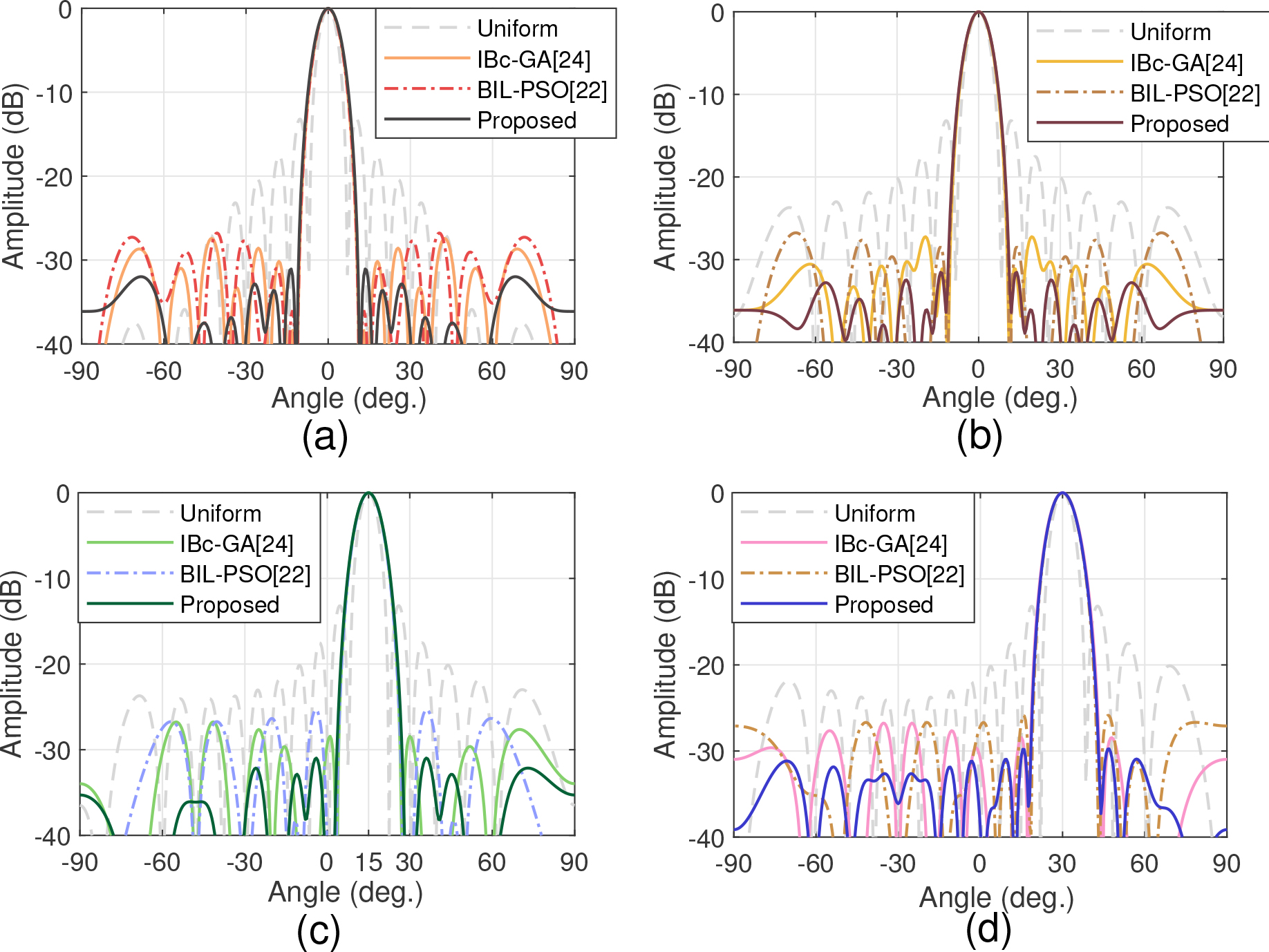
Figure 2: 2D far-field patterns of the 16 16 asymmetric planar array with a 50% fill factor. (a) Broadside pattern in = 0 plane. (b) Broadside pattern in = 90 plane. (c) Scanned pattern in = 0 plane with the main beam pointing at (= 15, = 0). (d) Scanned pattern in = 90 plane with the main beam pointing at (= 30, = 90).
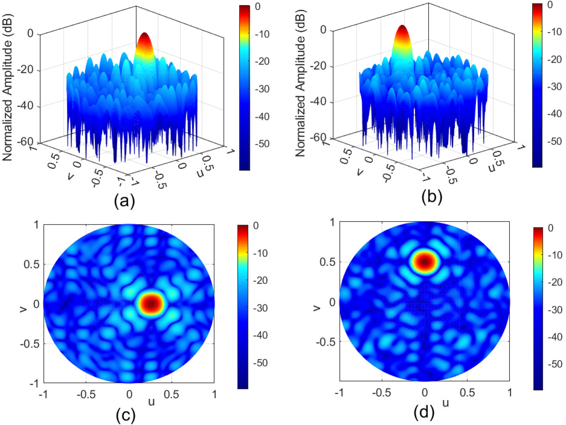
Figure 3: 3D far-field patterns of the 16 16 asymmetric planar array with a 50% fill factor. (a) and (c) Steering the main beam toward (= 15, = 0). (b) and (d) Steering the main beam toward (= 30, = 90).
Table 2: Comparison of the performance of thinned arrays using different algorithms when the main beam points at (= 0, = 0), (= 15, = 0), and (= 30, = 90)
| (, ) | Results | IBc-GA [24] | BIL-PSO [22] | 0-1 ILP |
| (0, 0) | PSLL (dB) ( = 0) | 26.72 | 27.40 | 31.04 |
| PSLL (dB) ( = 90) | 26.74 | 27.18 | 31.51 | |
| Direct. (dBi) | 25.42 | 25.63 | 25.80 | |
| (15, 0) | PSLL (dB) ( = 0) | 25.30 | 26.72 | 30.95 |
| Direct. (dBi) | 25.19 | 25.41 | 25.42 | |
| (30, 90) | PSLL (dB) ( = 90) | 25.84 | 26.73 | 29.74 |
| Direct. (dBi) | 25.11 | 25.06 | 25.15 |
B. Rectangular array design
In this case, a 20 10-element rectangular planar array was considered. In order to assess the performance of the 0-1 ILP technique, we attempted to replicate the methods published in [21–24] and compared the best results with those acquired by the proposed method. Table 3 gives the comparison between the optimization results obtained by methods in [21–23] and the 0-1 ILP algorithm. All of these methods were applied to a 20 10-element symmetric planar array, using fill factors from 54% to 68%. As shown in Table 3, the PSLLs obtained by OGA [21], BIL-PSO [22], and ACO [23] are nearly the same as the 0-1 ILP. However, the total optimization time of the proposed 0-1 ILP method is much shorter than that of other algorithms.
The performance comparisons of the IBc-GA [24], BIL-PSO [22], and 0-1 ILP in dealing with the 20 10-element asymmetric planar array with a 54% fill factor is presented in Table 4 and Figure 4. For a more accurate comparison, the FNBW values of these methods were controlled to be the same, where the FNBW in = 0 plane is set to 18 and the FNBW in = 90 plane is set to 36. The optimized element distributions obtained using the 0-1 ILP technique are illustrated in Figure 5. The white blocks in the figure represent the ON-state, and the black blocks represent the OFF-state. From Table 4, it can be seen that the maximum SLL in principal planes of the proposed approach is 28.55 dB, which is 2.11 dB lower than that achieved through IBc-GA [24] and 3.41 dB lower than that obtained by BIL-PSO [22]; yet, there is little difference in directivity. In addition, the total runtime of each algorithm is listed in the fourth row of Table 4. The average time for one execution of the proposed method is 0.47 s, and the total time for 30 independent runs is about 14.1 s, which is much less than the 3355.6 s required by IBc-GA in [24] and the 2835.4 s required by BIL-PSO in [22].
Table 3: Comparison of the PSLL and the total runtime of 20 10-element symmetric planar array synthesized with different algorithms
| Method | Filling factor | PSLL (dB) ( = 0) | PSLL (dB) ( = 90) | Total run time (s) |
| OGA [21] | 54.0% | 26.09 | 25.09 | 225.7 |
| 0-1 ILP | 54.0% | 26.09 | 25.09 | 8.9 |
| OGA [21] | 58.0% | 28.34 | 26.59 | 227.6 |
| BIL-PSO [22] | 58.0% | 28.31 | 26.57 | 241.5 |
| 0-1 ILP | 58.0% | 28.34 | 26.59 | 9.1 |
| ACO [23] | 68.0% | 25.67 | -25.76 | 326.8 |
| 0-1 ILP | 68.0% | 25.68 | 25.77 | 8.6 |
Table 4: Comparison of the performance of the 20 10 asymmetric planar array synthesized with the IBC-Ga [24], BIL-PSO [22], and 0-1 ILP methods
| Results | IBc-GA [24] | BIL-PSO [22] | 0-1 ILP |
|---|---|---|---|
| PSLL (dB) in = 0 plane |
26.64 | 25.14 | 28.55 |
| PSLL (dB) in = 90 plane |
26.44 | 25.44 | 29.37 |
| Directivity (dBi) | 25. 45 | 25.76 | 26.12 |
| Total run time (s) | 3355.6 | 2835.4 | 14.1 |
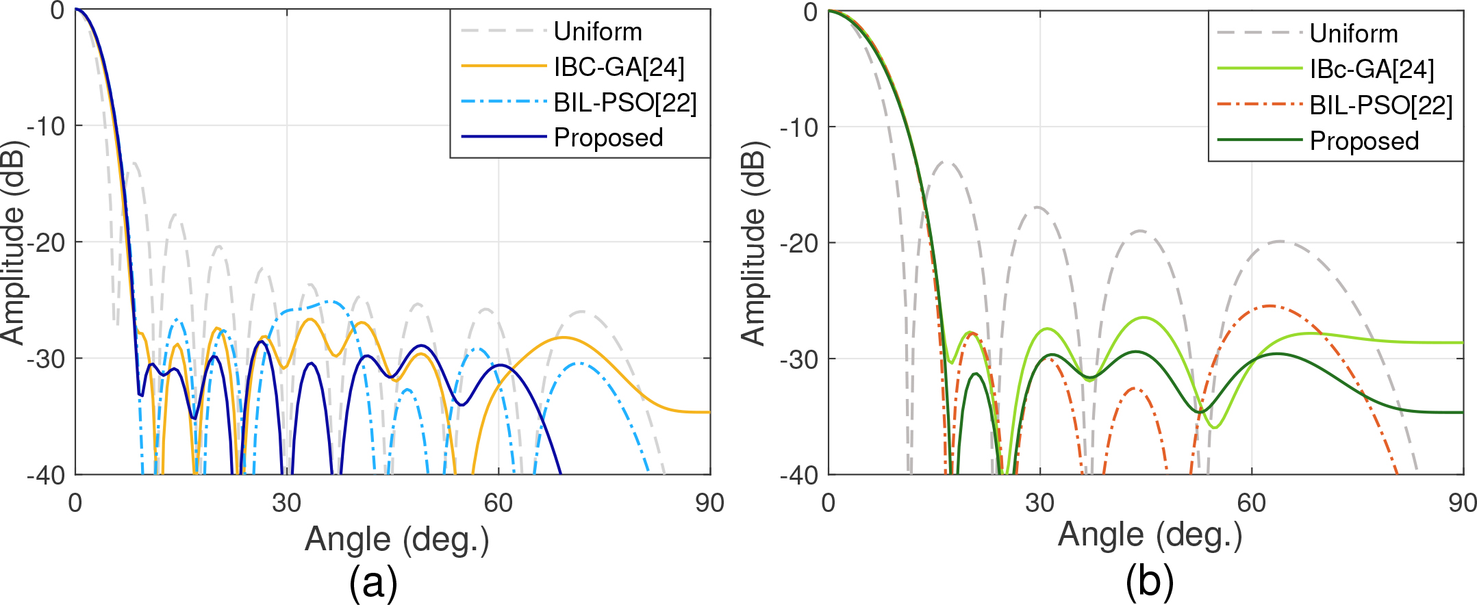
Figure 4: Far-field patterns of the 20 10 asymmetric planar array with a 54% fill factor obtained by uniform excitation, IBc-GA [24], BIL-PSO [22], and the proposed method. (a) 2D pattern in = 0 plane. (b) 2D pattern in = 90 plane.
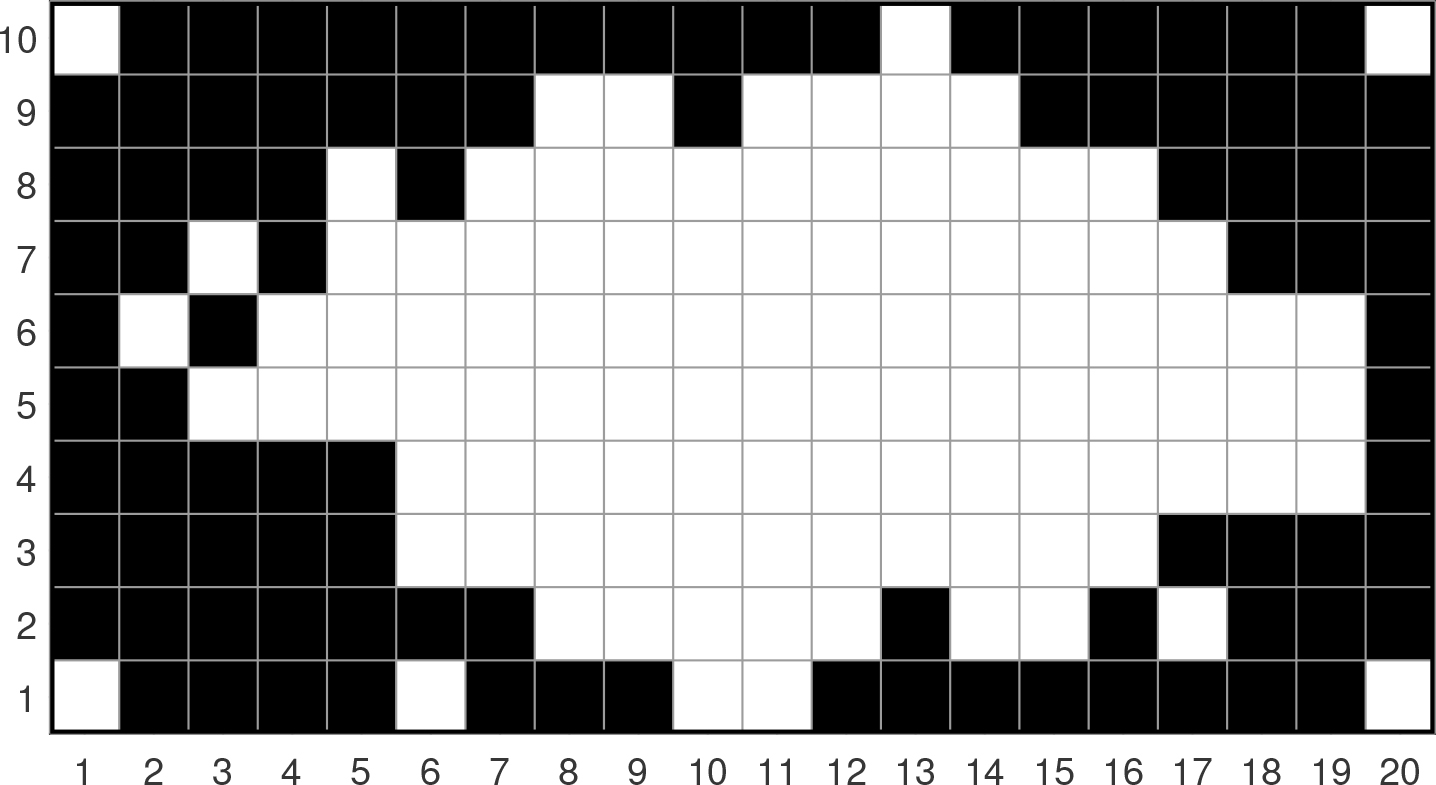
Figure 5: Distribution of the turned “ON” element across the 20 10 planar array with a 54% fill factor. White blocks indicate elements that are turned “ON” and black blocks indicate elements that are turned “OFF.”
Most papers on array thinning are devoted to optimizing symmetric arrays to reduce the solution space and speed up convergence. These algorithms show good performance in thinning small- and medium-scale symmetric antenna arrays and even achieve the global optimum. Yet, they can only end up with sub-optimal solutions when optimizing asymmetric planar arrays with equal size and the same total number of iterations. That may be because the asymmetric planar array has higher degrees of freedom, which increases the difficulty of optimization. However, our simulation results demonstrated that the 0-1 ILP algorithm outperforms [21–24] by achieving lower PSLL in a much shorter time.
C. Large-scale square array design
To investigate the capabilities of the 0-1 ILP method for thinning large-scale planar arrays, we considered a 100 100 symmetric planar square array with a 49.52% fill factor. The obtained results are given in Table 5 and Figures 68. Table 5 illustrates that the performance of the 0-1 ILP technique in optimizing PSLL is better than [25]. The peak SLL decreases from 32.80 to 40.88 dB in the = 0 plane and drops from 33.40 to 40.71 dB in the = 90 plane. The directivity of the thinned array is 40.18 dBi, and the FNBW in both = 0 plane and = 90 plane is 5. Figure 6 shows the 3D normalized far-field pattern, Figure 7 plots the 2D far-field pattern when = 0 and = 90, and Figure 8 gives the optimal distribution of the turned “ON” elements (white) and turned “OFF” elements (black) across the array aperture. The average time for one independent run of the proposed method is about 13.17 s, and the total time for 30 runs is about 395.1 s.
The high-dimensional optimization problem often comes with a considerable computational burden; so only a few published methods have the ability to synthesize large arrays. Although this method requires multiple adjustments of the parameters based on experience, the foregoing results and analysis demonstrated clearly that the 0-1 ILP method solves optimization problems with high-dimensional quickly and efficiently.
Table 5: Comparison of the PSLL of 100 100 square array designed with the IW-PSO [25] and 0-1 ILP approaches
| Results | IW-PSO [25] | 0-1 ILP |
|---|---|---|
| PSLL (dB) in = 0 plane | 32.80 | 40.88 |
| PSLL (dB)in = 90 plane | 33.40 | 40.71 |
| Directivity (dBi) | 40.18 | |
| Turned-ON elements | 4951 | 4952 |
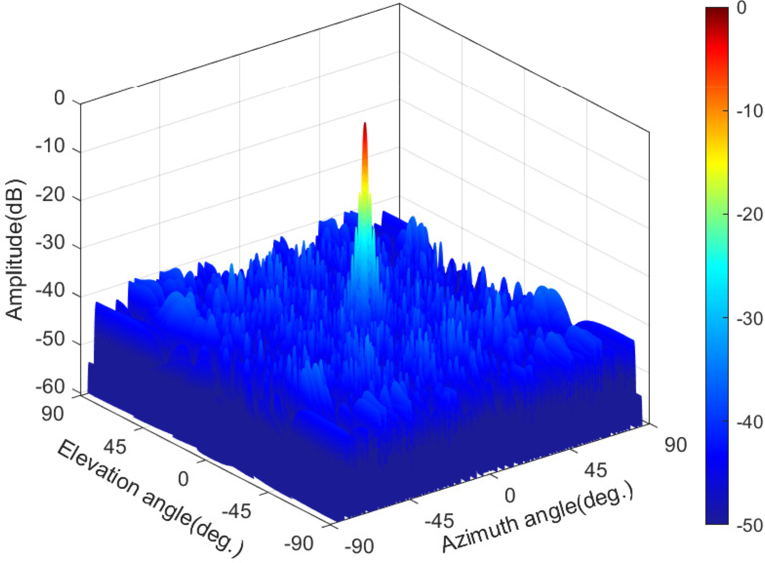
Figure 6: 3D pattern of the symmetric planar array consisting of 100 100 size and a 49.52% fill factor.
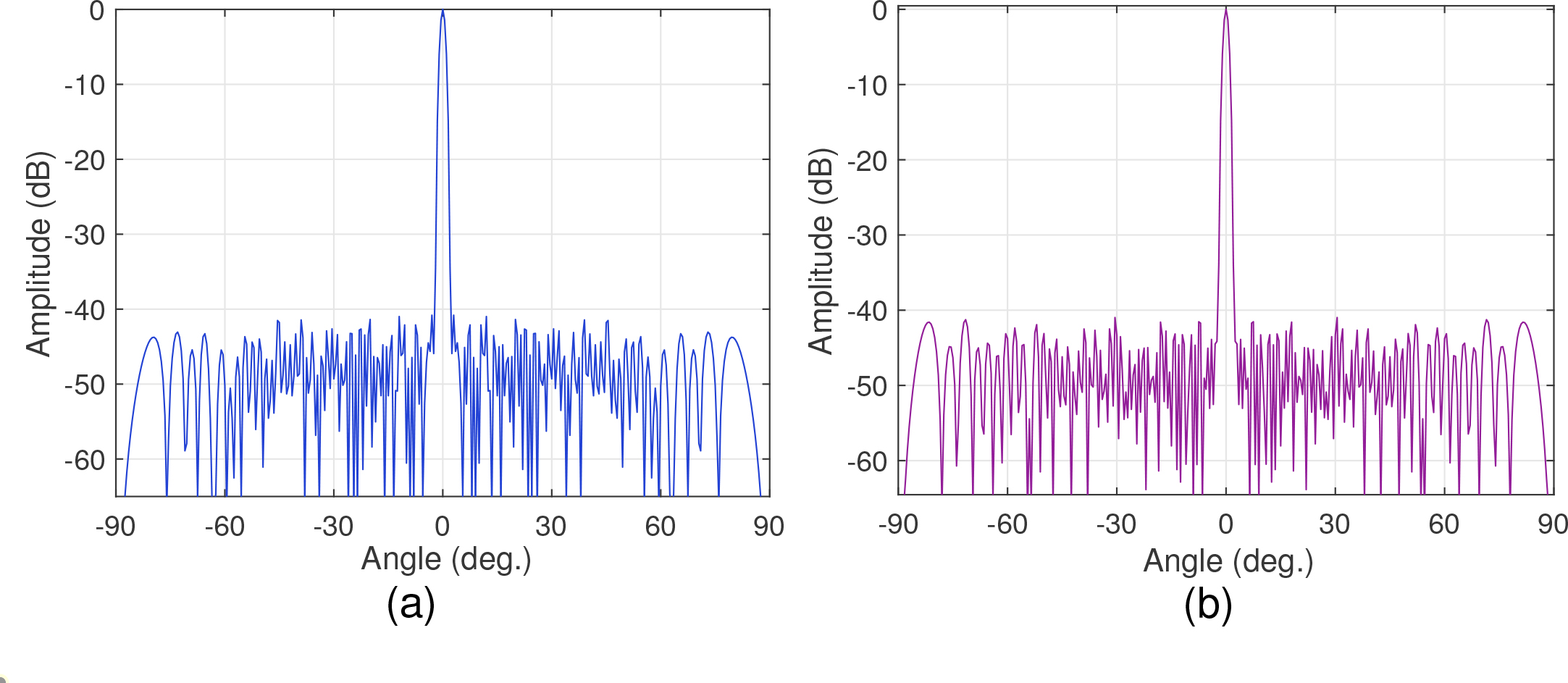
Figure 7: Far-field patterns of the 100 100 symmetric planar array with a 49.52% fill factor. (a) 2D pattern in = 0 plane. (b) 2D pattern in = 90 plane.
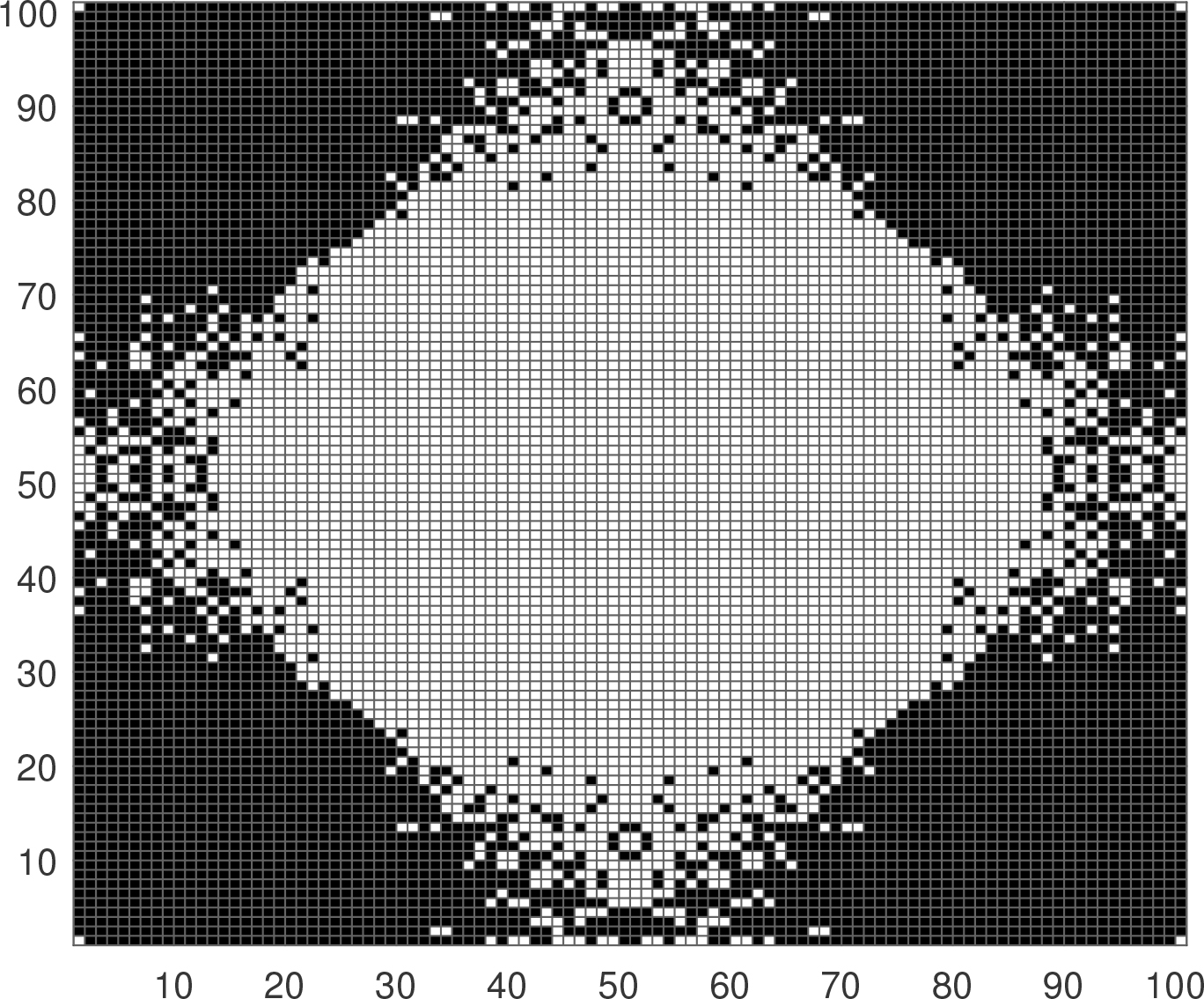
Figure 8: Distribution of the turned “ON” element across the 100 100 square array with a 49.52% fill factor. White blocks indicate elements that are turned “ON,” and black blocks indicate elements that are turned “OFF.”
D. Discussion of the results
Array thinning is a complex nonlinear problem and is difficult to be solved. Stochastic algorithms are computationally expensive, time-consuming, and may not converge to the optimal solution. In this paper, an approximate linearization technique was proposed to reduce the complexity of the model, which dramatically accelerates the calculation speed. The method is simple, efficient, and without any iterations. One drawback of the 0-1 ILP method is that the approximate linearization process may cause rounding errors. However, the numerical results evidenced that the linear programming model proposed in this paper has a high approximation accuracy, the optimizing result of which can be regarded as an approximate solution of the original model. Furthermore, since the solution accuracy of the intlinprog(.) function is limited, it could not get the optimal solution when optimizing larger arrays. Commercial optimization solvers such as Gurobi and CPLEX can be used to improve the solution accuracy of the 0-1 ILP model. The new approach has provided a novel strategy for thinning planar arrays, which has prominent advantages in solving the large-scale antenna array optimization problems with huge solution space and high complexity. In addition, it can be further applied to optimize the PSLL of the whole sidelobe region.
IV. CONCLUSION
This paper introduced the 0-1 ILP method for thinning planar arrays. The 0-1 ILP technique is a fast algorithm without iterative procedures. The obtained results of the new method were compared with some earlier published stochastic algorithms. Simulation results indicate that the method proposed in this paper can effectively suppress the peak SLL of planar arrays and substantially increase computational efficiency compared to the stochastic algorithm. Besides, we have successfully applied the method to optimize a beam-scannable antenna array and a 100 100 planar square array, demonstrating the effectiveness of the 0-1 ILP method for steerable arrays and large-scale array thinning, respectively. In future work, we will attempt to obtain lower PSLL in all planes and will further optimize the excitation current of the thinned planar arrays to reduce the PSLL by nonlinear programmingmethods.
REFERENCES
[1] R. L. Haupt, “Thinned arrays using genetic algorithms,” IEEE Trans. Antennas Propag., vol. 42, no. 7, pp. 993–999, Jul. 1994.
[2] N. Jin and Y. Rahmat-Samii, “Advances in particle swarm optimization for antenna designs: Real-number, binary, single-objective and multiobjective implementations,” IEEE Trans. Antennas Propag., vol. 55, no. 3, pp. 556–567, Mar. 2007.
[3] G. Sun, Y. Liu, Z. Chen, S. Liang, A. Wang, and Y. Zhang, “Radiation beam pattern synthesis of concentric circular antenna arrays using hybrid approach based on cuckoo search,” IEEE Trans. Antennas Propag., vol. 66, no. 9, pp. 4563–4576, Sep. 2018.
[4] A. S. Zare, S. Baghaiee. “Application of ant colony optimization algorithm to pattern synthesis of uniform circular antenna array”. Applied Computational Electromagnetics Society Journal, vol. 30, no. 8, pp. 810–818 Aug. 2015.
[5] S. Liang, Z. Fang, G. Sun, Y. Liu, G. Qu, and Y. Zhang, “Sidelobe reductions of antenna arrays via an improved chicken swarm optimization approach,” IEEE Access, vol. 8, pp. 37664–37683, 2020.
[6] R. E. Willey, “Space tapering of linear and planar arrays,” IRE Trans. Antennas Propag., vol. AP-10, no. 4, pp. 369–377, Jul. 1962.
[7] M. Skolnik, J. W. Sherman, III, and F. C. Ogg, Jr., “Statistically designed density-tapered arrays,” IEEE Trans. Antennas Propag., vol. AP-12, no. 4, pp. 408–417, Jul. 1964.
[8] O. M. Bucci, T. Isernia, and A. F. Morabito, “A deterministic approach to the synthesis of pencil beams through planar thinned arrays,” Prog. Electromagn. Res., vol. 101, no. 2, pp. 217–230, 2010.
[9] W. P. M. N. Keizer, “Linear array thinning using iterative FFT techniques,” IEEE Trans. Antennas Propag., vol. 56, no. 8, pp. 2260–2757, Aug. 2008.
[10] W. P. M. N. Keizer, “Large planar array thinning using iterative FFT techniques,” IEEE Trans. Antennas Propag., vol. 57, no. 10, pp. 3359–3362, Oct. 2009.
[11] M. Donelli, A. Martini, and A. Massa, “A hybrid approach based on PSO and Hadamard difference sets for the synthesis of square thinned arrays,” IEEE Trans. Antennas Propag., vol. 57, no. 8, pp. 2491–2495, Aug. 2009.
[12] G. Oliveri, L. Manica, and A. Massa, “ADS-based guidelines for thinned planar arrays,” IEEE Trans. Antennas Propag., vol. 58, no. 6, pp. 1935-1948, Jun. 2010.
[13] G. Oliveri, F. Caramanica, C. Fontanari, and A. Massa, “Rectangular thinned arrays based on McFarland difference sets,” IEEE Trans. Antennas Propag., vol. 59, no. 5, pp. 1546–1552, May 2011.
[14] P. Rocca, N. Anselmi, G. Oliveri, A. Polo and A. Massa, “Antenna array thinning through quantum Fourier transform,” IEEE Access, vol. 9, pp. 124313-124323, 2021.
[15] L. Gu, Y.-W. Zhao, Z.-P. Zhang, L.-F. Wu, Q.-M. Cai, and R.-R. Zhang, “Adaptive Learning of Probability Density taper for large planar array thinning,” IEEE Trans. Antennas Propag., vol. 69, no. 1, pp. 155-163, Jan. 2021.
[16] H. Xu, S. M. Conolly, G. C. Scott, and A. Macovski, “Homogeneous magnet design using linear programming,” IEEE Trans. Magn., vol. 36, no. 2, pp. 476–483, Mar. 2000.
[17] K. Yang, Z. Zhao, and Y. Liu, “Synthesis of sparse planar arrays with matrix pencil method,” in Proc. Int. Conf. on Computational Problem-Solving (ICCP), 2011, pp. 82–85.
[18] B. V. Ha, M. Mussetta, P. Pirinoli, and R. E. Zich, “Modified compact genetic algorithm for thinned array synthesis,” IEEE Antennas Wireless Propag. Lett., vol. 15, pp. 1105–1108, 2016.
[19] M. Jijenth, K. K. Suman, V. S. Gangwar, A. K. Singh, and S. P. Singh, “A novel technique based on modified genetic algorithm for the synthesis of thinned planar antenna array with low peak sidelobe level over desired scan volume,” in IEEE MTT-S International Microwave and RF Conference (IMaRC), Dec 2017, pp. 251–254.
[20] K. V. Deligkaris, Z. D. Zaharis, D. G. Kampitaki, S. K. Goudos, I. T. Rekanos, and M. N. Spasos, “Thinned planar array design using Boolean PSO with velocity mutation,” IEEE Trans Magn., vol. 45, no. 3, pp. 1490-1493, Mar. 2009.
[21] L. Zhang, Y.-C. Jiao, B. Chen, and H. Li, “Orthogonal genetic algorithm for planar thinned array designs,” International Journal of Antennas and Propagation, vol. 2012, 2012.
[22] D. Liu, Q. Jiang, and J. X. Chen, “Binary inheritance learning particle swarm optimisation and its application in thinned antenna array synthesis with the minimum sidelobe level,” IET Microw., Antennas Propag., vol. 9, no. 13, pp. 1386–1391, 2015.
[23] O. Quevedo-Teruel and E. Rajo-Iglesias, “Ant colony optimization in thinned array synthesis with minimum sidelobe level,” IEEE Antennas Wireless Propag. Lett., vol. 5, pp. 349–352, 2006.
[24] V. S. Gangwar, R. K. Samminga, A. K. Singh, M. Jijenth, K. K. Suman, and S. P. Singh, “A novel strategy for the synthesis of thinned planar antenna array which furnishes lowest possible peak sidelobe level without appearance of grating lobes over wide steering angles”, Journal of Electromagnetic Waves and Applications, 2017,pp. 842-857.
[25] J. K. Modi, R. K. Gangwar, P. Ashwin and V. S. Gangwar, ”An efficious strategy for the synthesis of large arrays thinning with low PSLL,” 2019 International Conference on Wireless Communications Signal Processing and Networking (WiSPNET), 2019, pp. 41-43.
BIOGRAPHIES

Mingyu Wang was born in Hohhot, Inner Mongolia Autonomous Region, China. She received the B.S. degree in communication engineering from Hohai University, Nanjing, China, in 2019. She is currently working toward the master’s degree in signal and information processing with the same university.
Her research interests include the design of antenna arrays.

Xuewei Ping was born in Hebi of He’nan Province, China. He received the Ph.D. degree in electromagnetic field and microwave technology from the Nanjing University of Science and Technology, Nanjing, China, in 2007.
He is currently with the College of Computer and Information, Hohai University, Nanjing, China. His research interests include computational electromagnetics and the design and analysis of superconducting magnets and gradient coils.
ACES JOURNAL, Vol. 37, No. 2, 191–198.
doi: 10.13052/2022.ACES.J.370207
© 2021 River Publishers