Prediction and Analysis of the Shielding Effectiveness and Resonances of a Cascaded Triple Enclosure Based on Electromagnetic Topology

Jin-Cheng Zhou and Xue-Tian Wang

¹School of Information and Electronics, Beijing Institute of Technology, Beijing 100081, China
zjc.chn@gmail.com, wangxuetian@bit.edu.cn

Submitted On: December 16, 2021; Accepted On: March 11, 2022

Abstract

A fast analytical method for predicting the shielding effectiveness (SE) and resonances of a parallelly–serially cascaded triple enclosure was proposed. Under the concept of electromagnetic topology, the observation points and the walls are treated as nodes and the space between them as tubes. An equivalent circuit model of the enclosures is derived in which the apertures on the front and rear walls of the two parallelly cascaded sub-enclosures are considered as a pair of three-port networks. To predict the SE at a particular monitoring point, we introduce the position factor. The results of the proposed method have a good agreement with the numerical methods while it is much faster. The proposed method can help in determining SE for cascaded enclosures. We can also find that the resonance effect affects each subenclosure through the apertures, which must be carefully considered inpractice.

Keywords: Shielding effectiveness, aperture coupling, general Baum–Liu–Tesche equation

I. INTRODUCTION

The development of high-power microwave (HPM), such as radar illuminating and electromagnetic pulses, in recent years has the potential to damage digital systems. Electromagnetic shielding is one of the most commonly used techniques to protect valuable electronics. The shielding performance of an enclosure with apertures is defined by the shielding effectiveness (SE), which is the ratio of the electric field at an observation point without and with the enclosure [1].

There are numerous approaches for calculating SE of the shielding enclosures with apertures, which can generally be divided into numerical methods and analytical formulations.

Numerical methods include finite-difference time-domain method [2], method of moments [3, 4], transmission line matrix (TLM) method [5]. Numerical methods can handle complicated structures, but they often consume more computational resources.

The analytical formulations are based on circuit models. For instance, Robinson’s method [6, 7] and its developed methods [8, 9, 10, 11] are based on transmission line parameters. In this type of method, the rectangular enclosure and the aperture are modeled by a short-circuited rectangular waveguide and a transmission line, respectively. However, the analytical formulations can hardly handle complex enclosure structures.

Electromagnetic topology (EMT) provides a useful tool for studying the coupling problems of complicated electrical systems, which treat the complex interaction problem into smaller and more manageable problems [12, 13]. By applying the EMT concept, the Baum–Liu–Tesche (BLT) equation can be derived to calculate the voltage and current responses at the nodes of a general multiconductor transmission line network. After transforming the enclosure and aperture into nodes, we can use the extended BLT equation to calculate the voltage and current at all nodes [14, 15]. In [16], a method is proposed to use the BLT equation to predict the SE of multiple cascaded enclosures, but the monitoring points are limited to the center axis of eachfront wall.

In this paper, we propose a fast algorithm based on the EMT to predict the SE for a parallelly–serially cascaded triple enclosure. The SE and resonances at any monitor point can be quickly and effectively predicted over a wide bandwidth range by introducing the aperture position factor.

The structure of this paper is as follows. The electromagnetic topological model and equivalent circuit are given along with the derivation of the extended BLT equation in Section 2. Validation of the model is given in Section 3, and Section 4 summarizes the conclusions of this paper.

II. ELECTROMAGNETIC TOPOLOGICAL MODEL

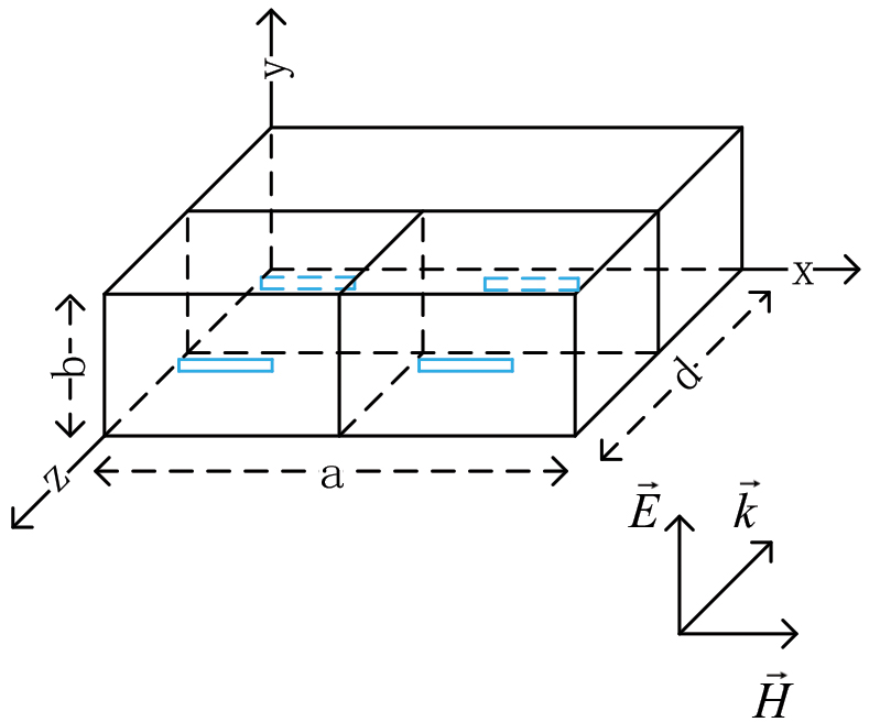
Figure 1: Rectangular parallelly–serially cascaded enclosure and its coordinate system; all apertures are positioned centrally in the walls.

In this paper, we focus on a parallelly–serially cascaded triple enclosure. The structure of this enclosure is shown in Figure 1. The overall size of the enclosure is $300\times 100\times 500$ mm, and the thickness of the enclosure wall is 1 mm.

The enclosure consists of three enclosures, and the subenclosure of the left-front one in Figure 1 is labeled as number 1 and has size $c\times b\times d_1$. The one on the right is labeled as number 2 and has the same size as Enclosure 1. And the rear one is labeled as number 3, and the size is $a\times b\times d_2$; it is also the biggest sub-enclosure. The left aperture $a{p}_1$ at the front wall of Enclosure 1 has a dimension of $l_1\times w_1$ and the right aperture $a{p}_2$ has a dimension of $l_2\times w_2$, and another pair of apertures $a{p}_3$ and $a{p}_4$ with dimensions $l_3\times w_3$ and $l_4\times w_4$ are located on the second wall. $P_1$, $P_2$, and $P_3$ are observation points located in the center of each subenclosure,respectively.

The equivalent circuit of the cascaded enclosures in Figure 1 is given in Figure 2. The impedance and propagation constants $z_g$ and $k_g$ are given by

$$k_g=k_0\sqrt{1-{\left(\frac{m\lambda }{2a}\right)}^2-{\left(\frac{n\lambda }{2b}\right)}^2}$$

(1)

$$Z_g=Z_0/\sqrt{1-{\left(\frac{m\lambda }{2a}\right)}^2-{\left(\frac{n\lambda }{2b}\right)}^2}.$$

(2)

The radiating source is represented by voltage $V_0$ and impedance of free space $Z_0=377\mathrm{\Omega }$. Aperture is treated as a coplanar strip transmission line which is shorted at each end; its characteristic impedance is given by Gupta et al [17]:

$$Z_{ap}=C_a\frac{j}{2}\frac{l}{a}{Z}_{os}\tan \left(\frac{{\mathrm{k}}_0\mathrm{l}}{2}\right).$$

(3)

$C_a$ is the position factor which is defined as [8, 11]

$$C_a=\sin \left(\frac{\mathrm{m}\pi }{\mathrm{a}}{\mathrm{x}}_{\mathrm{a}}\right)\cos \left(\frac{\mathrm{n}\pi }{\mathrm{b}}{\mathrm{y}}_{\mathrm{a}}\right).$$

(4)

$x_a$ and $y_a$ are the position coordinate, and $m$ and $n$ are mode indices. We can find that when the aperture is located at the center of the wall, $T{E}_{01}$, $T{M}_{11}$, and $T{E}_{20}$ modes will not exist.

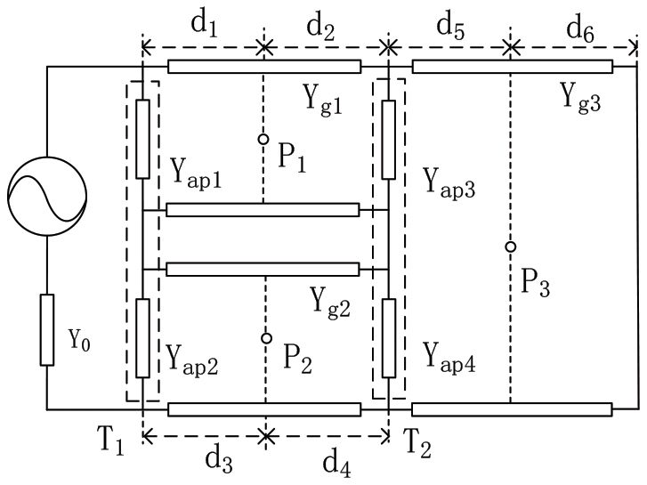
Figure 2: Equivalent circuit of the parallelly–serially cascaded enclosure.

Since the cascaded enclosures have a thickness, we have effective width $w_e$

$$w_e=w-\frac{5t}{4\pi }\left[1+\ln \frac{4\pi w}{t}\right]$$

(5)

where $t$ is the thickness of the enclosure’s wall and $w$ is the width of the aperture. If the shape of the aperture is close to a slot ($w_e⩽\frac{b}{\sqrt{2}}$), we have

$$Z_{os}=120{\pi }^2\left[\ln \left(2\frac{1+\sqrt[4]{1-{(w_e/b)}^2}}{1-\sqrt[4]{1-{(w_e/b)}^2}}\right)\right].$$

(6)

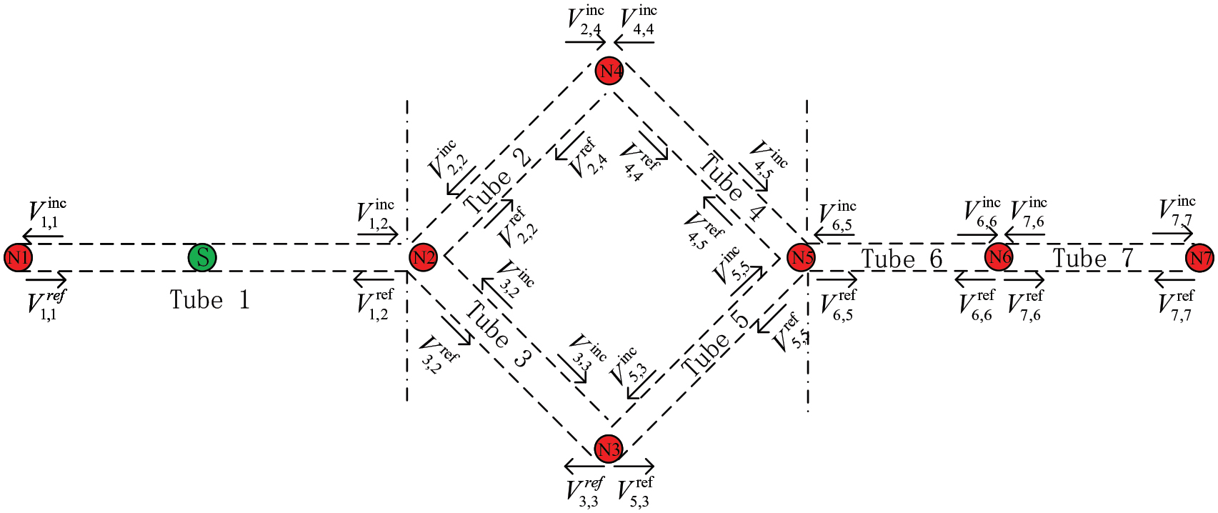
Figure 3: Signal flow graph of cascaded enclosures.

$$\left[\begin{array}{c}\hfill V_{1,1}^r\hfill \\ \hfill V_{1,2}^r\hfill \\ \hfill V_{2,2}^r\hfill \\ \hfill V_{3,2}^r\hfill \\ \hfill V_{3,3}^r\hfill \\ \hfill V_{5,3}^r\hfill \\ \hfill V_{2,4}^r\hfill \\ \hfill V_{4,4}^r\hfill \\ \hfill V_{4,5}^r\hfill \\ \hfill V_{5,5}^r\hfill \\ \hfill V_{6,5}^r\hfill \\ \hfill V_{6,6}^r\hfill \\ \hfill V_{7,6}^r\hfill \\ \hfill V_{7,7}^r\hfill \end{array}\right]=\left[\begin{array}{cccccccccccccc}\hfill 0\hfill & \hfill e^{{\gamma }_0{l}_x}\hfill & \hfill 0\hfill & \hfill 0\hfill & \hfill 0\hfill & \hfill 0\hfill & \hfill 0\hfill & \hfill 0\hfill & \hfill 0\hfill & \hfill 0\hfill & \hfill 0\hfill & \hfill 0\hfill & \hfill 0\hfill & \hfill 0\hfill \\ \hfill e^{{\gamma }_0{l}_x}\hfill & \hfill 0\hfill & \hfill 0\hfill & \hfill 0\hfill & \hfill 0\hfill & \hfill 0\hfill & \hfill 0\hfill & \hfill 0\hfill & \hfill 0\hfill & \hfill 0\hfill & \hfill 0\hfill & \hfill 0\hfill & \hfill 0\hfill & \hfill 0\hfill \\ \hfill 0\hfill & \hfill 0\hfill & \hfill 0\hfill & \hfill 0\hfill & \hfill 0\hfill & \hfill 0\hfill & \hfill e^{T_1}\hfill & \hfill 0\hfill & \hfill 0\hfill & \hfill 0\hfill & \hfill 0\hfill & \hfill 0\hfill & \hfill 0\hfill & \hfill 0\hfill \\ \hfill 0\hfill & \hfill 0\hfill & \hfill 0\hfill & \hfill 0\hfill & \hfill e^{T_3}\hfill & \hfill 0\hfill & \hfill 0\hfill & \hfill 0\hfill & \hfill 0\hfill & \hfill 0\hfill & \hfill 0\hfill & \hfill 0\hfill & \hfill 0\hfill & \hfill 0\hfill \\ \hfill 0\hfill & \hfill 0\hfill & \hfill 0\hfill & \hfill e^{T_3}\hfill & \hfill 0\hfill & \hfill 0\hfill & \hfill 0\hfill & \hfill 0\hfill & \hfill 0\hfill & \hfill 0\hfill & \hfill 0\hfill & \hfill 0\hfill & \hfill 0\hfill & \hfill 0\hfill \\ \hfill 0\hfill & \hfill 0\hfill & \hfill 0\hfill & \hfill 0\hfill & \hfill 0\hfill & \hfill 0\hfill & \hfill 0\hfill & \hfill 0\hfill & \hfill 0\hfill & \hfill e^{T_4}\hfill & \hfill 0\hfill & \hfill 0\hfill & \hfill 0\hfill & \hfill 0\hfill \\ \hfill 0\hfill & \hfill 0\hfill & \hfill e^{T_1}\hfill & \hfill 0\hfill & \hfill 0\hfill & \hfill 0\hfill & \hfill 0\hfill & \hfill 0\hfill & \hfill 0\hfill & \hfill 0\hfill & \hfill 0\hfill & \hfill 0\hfill & \hfill 0\hfill & \hfill 0\hfill \\ \hfill 0\hfill & \hfill 0\hfill & \hfill 0\hfill & \hfill 0\hfill & \hfill 0\hfill & \hfill 0\hfill & \hfill 0\hfill & \hfill 0\hfill & \hfill e^{T_2}\hfill & \hfill 0\hfill & \hfill 0\hfill & \hfill 0\hfill & \hfill 0\hfill & \hfill 0\hfill \\ \hfill 0\hfill & \hfill 0\hfill & \hfill 0\hfill & \hfill 0\hfill & \hfill 0\hfill & \hfill 0\hfill & \hfill 0\hfill & \hfill e^{T_2}\hfill & \hfill 0\hfill & \hfill 0\hfill & \hfill 0\hfill & \hfill 0\hfill & \hfill 0\hfill & \hfill 0\hfill \\ \hfill 0\hfill & \hfill 0\hfill & \hfill 0\hfill & \hfill 0\hfill & \hfill 0\hfill & \hfill e^{T_4}\hfill & \hfill 0\hfill & \hfill 0\hfill & \hfill 0\hfill & \hfill 0\hfill & \hfill 0\hfill & \hfill 0\hfill & \hfill 0\hfill & \hfill 0\hfill \\ \hfill 0\hfill & \hfill 0\hfill & \hfill 0\hfill & \hfill 0\hfill & \hfill 0\hfill & \hfill 0\hfill & \hfill 0\hfill & \hfill 0\hfill & \hfill 0\hfill & \hfill 0\hfill & \hfill 0\hfill & \hfill e^{T_5}\hfill & \hfill 0\hfill & \hfill 0\hfill \\ \hfill 0\hfill & \hfill 0\hfill & \hfill 0\hfill & \hfill 0\hfill & \hfill 0\hfill & \hfill 0\hfill & \hfill 0\hfill & \hfill 0\hfill & \hfill 0\hfill & \hfill 0\hfill & \hfill e^{T_5}\hfill & \hfill 0\hfill & \hfill 0\hfill & \hfill 0\hfill \\ \hfill 0\hfill & \hfill 0\hfill & \hfill 0\hfill & \hfill 0\hfill & \hfill 0\hfill & \hfill 0\hfill & \hfill 0\hfill & \hfill 0\hfill & \hfill 0\hfill & \hfill 0\hfill & \hfill 0\hfill & \hfill 0\hfill & \hfill 0\hfill & \hfill e^{T_6}\hfill \\ \hfill 0\hfill & \hfill 0\hfill & \hfill 0\hfill & \hfill 0\hfill & \hfill 0\hfill & \hfill 0\hfill & \hfill 0\hfill & \hfill 0\hfill & \hfill 0\hfill & \hfill 0\hfill & \hfill 0\hfill & \hfill 0\hfill & \hfill e^{T_6}\hfill & \hfill 0\hfill \end{array}\right]\left[\begin{array}{c}\hfill V_{1,1}^i\hfill \\ \hfill V_{1,2}^i\hfill \\ \hfill V_{2,2}^i\hfill \\ \hfill V_{3,2}^i\hfill \\ \hfill V_{3,3}^i\hfill \\ \hfill V_{5,3}^i\hfill \\ \hfill V_{2,4}^i\hfill \\ \hfill V_{4,4}^i\hfill \\ \hfill V_{4,5}^i\hfill \\ \hfill V_{5,5}^i\hfill \\ \hfill V_{6,5}^i\hfill \\ \hfill V_{6,6}^i\hfill \\ \hfill V_{7,6}^i\hfill \\ \hfill V_{7,7}^i\hfill \end{array}\right]-\left[\begin{array}{c}\hfill V_0\hfill \\ \hfill 0\hfill \\ \hfill 0\hfill \\ \hfill 0\hfill \\ \hfill 0\hfill \\ \hfill 0\hfill \\ \hfill 0\hfill \\ \hfill 0\hfill \\ \hfill 0\hfill \\ \hfill 0\hfill \\ \hfill 0\hfill \\ \hfill 0\hfill \\ \hfill 0\hfill \\ \hfill 0\hfill \end{array}\right].$$

(7)

Figure 3 gives EMT for the triple enclosures shown in Figure 1. Node $N_1$ represents the observation point outside the enclosure which is equivalented by one-port network; nodes $N_3$, $N_4$, and $N_6$ denote observation points $P_1$, $P_2$, and $P_3$ inside the subenclosures respectively, and they are equivalented by two-port networks. The apertures are represented by nodes $N_2$ and $N_5$ as three-port network, and the shorted end is represented by $N_7$ as one-port network. Tube 1 denotes the electromagnetic wave propagation in free space, while Tube 2, Tube 3, Tube 4, Tube 5, and Tube 6 are the wave propagation between the observation points and the apertures in subenclosures. Tube 7 denotes the wave propagation to the short end of Enclosure 3.

As illustrated by Figure 3, we have a propagation matrix as shown in eqn (7):

$l_x$ is the distance between electromagnetic wave and the apertures; ${\gamma }_0=j{k}_0$ is the phase constant of freespace. $T_i$ represents the phase constant of each subenclosure:

$$T_1={\gamma }_{g1}{d}_1,T_2={\gamma }_{g1}{d}_2$$

(8)

$$T_3={\gamma }_{g2}{d}_3,T_4={\gamma }_{g2}{d}_4$$

(9)

$$T_5={\gamma }_{g3}{d}_5,T_6={\gamma }_{g3}{d}_6.$$

(10)

Here, ${\gamma }_g=j{k}_0\sqrt{1-{(m\lambda /2a)}^2-{(n\lambda /2b)}^2}$, and $d_i$ shown in Figure 2 represents the distance between each point in the planar wave propagation direction. We can also write eqn (7) as

$${\mathbf{V}}^{\mathbf{ref}}=\mathrm{\Gamma }\times {\mathbf{V}}^{\mathbf{inc}}-{\mathbf{V}}_{\mathbf{s}}.$$

(11)

The scattering matrix S contains the scattering coefficients as shown in eqn (12). For the responses ordered by the tube number, this matrix is sparse, but not necessarily block diagonal, since the locations of the various scattering coefficients depend on how the junctions in the network are numbered and interconnected:

$$\left[\begin{array}{c}\hfill V_{1,1}^r\hfill \\ \hfill V_{1,2}^r\hfill \\ \hfill V_{2,2}^r\hfill \\ \hfill V_{3,2}^r\hfill \\ \hfill V_{3,3}^r\hfill \\ \hfill V_{5,3}^r\hfill \\ \hfill V_{2,4}^r\hfill \\ \hfill V_{4,4}^r\hfill \\ \hfill V_{4,5}^r\hfill \\ \hfill V_{5,5}^r\hfill \\ \hfill V_{6,5}^r\hfill \\ \hfill V_{6,6}^r\hfill \\ \hfill V_{7,6}^r\hfill \\ \hfill V_{7,7}^r\hfill \end{array}\right]=\left[\begin{array}{cccccccccccccc}\hfill {\rho }^1\hfill & \hfill 0\hfill & \hfill 0\hfill & \hfill 0\hfill & \hfill 0\hfill & \hfill 0\hfill & \hfill 0\hfill & \hfill 0\hfill & \hfill 0\hfill & \hfill 0\hfill & \hfill 0\hfill & \hfill 0\hfill & \hfill 0\hfill & \hfill 0\hfill \\ \hfill 0\hfill & \hfill S_{11}^2\hfill & \hfill S_{12}^2\hfill & \hfill S_{13}^2\hfill & \hfill 0\hfill & \hfill 0\hfill & \hfill 0\hfill & \hfill 0\hfill & \hfill 0\hfill & \hfill 0\hfill & \hfill 0\hfill & \hfill 0\hfill & \hfill 0\hfill & \hfill 0\hfill \\ \hfill 0\hfill & \hfill S_{21}^2\hfill & \hfill S_{22}^2\hfill & \hfill S_{23}^2\hfill & \hfill 0\hfill & \hfill 0\hfill & \hfill 0\hfill & \hfill 0\hfill & \hfill 0\hfill & \hfill 0\hfill & \hfill 0\hfill & \hfill 0\hfill & \hfill 0\hfill & \hfill 0\hfill \\ \hfill 0\hfill & \hfill S_{31}^2\hfill & \hfill S_{32}^2\hfill & \hfill S_{33}^2\hfill & \hfill 0\hfill & \hfill 0\hfill & \hfill 0\hfill & \hfill 0\hfill & \hfill 0\hfill & \hfill 0\hfill & \hfill 0\hfill & \hfill 0\hfill & \hfill 0\hfill & \hfill 0\hfill \\ \hfill 0\hfill & \hfill 0\hfill & \hfill 0\hfill & \hfill 0\hfill & \hfill S_{11}^3\hfill & \hfill S_{12}^3\hfill & \hfill 0\hfill & \hfill 0\hfill & \hfill 0\hfill & \hfill 0\hfill & \hfill 0\hfill & \hfill 0\hfill & \hfill 0\hfill & \hfill 0\hfill \\ \hfill 0\hfill & \hfill 0\hfill & \hfill 0\hfill & \hfill 0\hfill & \hfill S_{21}^3\hfill & \hfill S_{22}^3\hfill & \hfill 0\hfill & \hfill 0\hfill & \hfill 0\hfill & \hfill 0\hfill & \hfill 0\hfill & \hfill 0\hfill & \hfill 0\hfill & \hfill 0\hfill \\ \hfill 0\hfill & \hfill 0\hfill & \hfill 0\hfill & \hfill 0\hfill & \hfill 0\hfill & \hfill 0\hfill & \hfill S_{11}^4\hfill & \hfill S_{12}^4\hfill & \hfill 0\hfill & \hfill 0\hfill & \hfill 0\hfill & \hfill 0\hfill & \hfill 0\hfill & \hfill 0\hfill \\ \hfill 0\hfill & \hfill 0\hfill & \hfill 0\hfill & \hfill 0\hfill & \hfill 0\hfill & \hfill 0\hfill & \hfill S_{21}^4\hfill & \hfill S_{22}^4\hfill & \hfill 0\hfill & \hfill 0\hfill & \hfill 0\hfill & \hfill 0\hfill & \hfill 0\hfill & \hfill 0\hfill \\ \hfill 0\hfill & \hfill 0\hfill & \hfill 0\hfill & \hfill 0\hfill & \hfill 0\hfill & \hfill 0\hfill & \hfill 0\hfill & \hfill 0\hfill & \hfill S_{11}^5\hfill & \hfill S_{12}^5\hfill & \hfill S_{13}^5\hfill & \hfill 0\hfill & \hfill 0\hfill & \hfill 0\hfill \\ \hfill 0\hfill & \hfill 0\hfill & \hfill 0\hfill & \hfill 0\hfill & \hfill 0\hfill & \hfill 0\hfill & \hfill 0\hfill & \hfill 0\hfill & \hfill S_{21}^5\hfill & \hfill S_{22}^5\hfill & \hfill S_{23}^5\hfill & \hfill 0\hfill & \hfill 0\hfill & \hfill 0\hfill \\ \hfill 0\hfill & \hfill 0\hfill & \hfill 0\hfill & \hfill 0\hfill & \hfill 0\hfill & \hfill 0\hfill & \hfill 0\hfill & \hfill 0\hfill & \hfill S_{31}^5\hfill & \hfill S_{32}^5\hfill & \hfill S_{33}^5\hfill & \hfill 0\hfill & \hfill 0\hfill & \hfill 0\hfill \\ \hfill 0\hfill & \hfill 0\hfill & \hfill 0\hfill & \hfill 0\hfill & \hfill 0\hfill & \hfill 0\hfill & \hfill 0\hfill & \hfill 0\hfill & \hfill 0\hfill & \hfill 0\hfill & \hfill 0\hfill & \hfill S_{11}^6\hfill & \hfill S_{12}^6\hfill & \hfill 0\hfill \\ \hfill 0\hfill & \hfill 0\hfill & \hfill 0\hfill & \hfill 0\hfill & \hfill 0\hfill & \hfill 0\hfill & \hfill 0\hfill & \hfill 0\hfill & \hfill 0\hfill & \hfill 0\hfill & \hfill 0\hfill & \hfill S_{21}^6\hfill & \hfill S_{22}^6\hfill & \hfill 0\hfill \\ \hfill 0\hfill & \hfill 0\hfill & \hfill 0\hfill & \hfill 0\hfill & \hfill 0\hfill & \hfill 0\hfill & \hfill 0\hfill & \hfill 0\hfill & \hfill 0\hfill & \hfill 0\hfill & \hfill 0\hfill & \hfill 0\hfill & \hfill 0\hfill & \hfill {\rho }^6\hfill \end{array}\right]\left[\begin{array}{c}\hfill V_{1,1}^i\hfill \\ \hfill V_{1,2}^i\hfill \\ \hfill V_{2,2}^i\hfill \\ \hfill V_{3,2}^i\hfill \\ \hfill V_{3,3}^c\hfill \\ \hfill V_{5,3}^i\hfill \\ \hfill V_{2,4}^i\hfill \\ \hfill V_{4,4}^i\hfill \\ \hfill V_{4,5}^i\hfill \\ \hfill V_{5,5}^i\hfill \\ \hfill V_{6,5}^i\hfill \\ \hfill V_{6,6}^i\hfill \\ \hfill V_{7,6}^i\hfill \\ \hfill V_{7,7}^i\hfill \end{array}\right].$$

(12)

${\rho }^1=0$ is the free space, and ${\rho }^6=-1$ is the short end of the Enclosure 3. $S^3$ , $S^4$, and $S^5$ represent $P_1$, $P_2$, and $P_3$:

$$S^3=S^4=S^6=\left[\begin{array}{cc}\hfill 0\hfill & \hfill 1\hfill \\ \hfill 1\hfill & \hfill 0\hfill \end{array}\right].$$

(13)

$S^2$ and $S^5$ can be obtained from network $T_1$ and $T_2$in Figure 2 respectively. Since the apertures are orthogonal to the propagation direction, we cannot determine the transmission between them; so we neglect the coupling between aperture 1 and aperture 2 and, hence, $S_{23}^2=S_{32}^2=0$:

$S_{11}^2=\text{(}{Y}_0{Y}_{g2}+Y_0{Y}_{ap2}+Y_0{Y}_{ap1}+Y_0{Y}_{g1}-Y_{g1}{Y}_{g2}-Y_{g1}{Y}_{ap2}-Y_{g2}{Y}_{ap1}-Y_{ap1}{Y}_{ap2})/Y{}_t{}^2$

$S_{12}^2=2(Y_0{Y}_{g2}+Y_0{Y}_{ap2})/Y_t^2$

$S_{13}^2=2(Y_0{Y}_{g1}+Y_0{Y}_{ap1})/Y_t^2$

$S_{21}^2=2(Y_0{Y}_{g1}+Y_{g1}{Y}_{g2}+Y_{g1}{Y}_{ap2})/Y_t^2$

$S_{22}^2=(Y_0{Y}_{g1}+Y_{g1}{Y}_{g2}+Y_{g1}{Y}_{ap2}-Y_0{Y}_{ap1}-Y_{g2}{Y}_{ap1}-Y_{ap1}{Y}_{ap2}-Y_0{Y}_{ap2}-Y_0{Y}_{g2})/Y_t^2$

$S_{31}^2=2(Y_0{Y}_{g2}+Y_{g1}{Y}_{g2}+Y_{g2}{Y}_{ap1})/Y_t^2$

$S_{33}^2=Y_0{Y}_{g2}+Y_{g1}{Y}_{g2}+Y_{g2}{Y}_{ap1}-Y_0{Y}_{ap2}-Y_{g1}{Y}_{ap2}-Y_0{Y}_{ap2}-Y_0{Y}_{g1}-Y_{ap1}{Y}_{ap2}$

$Y_t^2=Y_0{Y}_{g2}+Y_0{Y}_{ap2}+Y_0{Y}_{ap1}+Y_0{Y}_{g1}+Y_{g1}{Y}_{g2}+Y_{g1}{Y}_{ap2}+Y_{g2}{Y}_{ap1}+Y_{ap1}{Y}_{ap2}$.

For the same reason mentioned above, $S_{12}^5=$$S_{21}^5=0$:

$S_{11}^5=(Y_{g1}{Y}_{g3}+Y_{g1}{Y}_{g2}+Y_{g1}{Y}_{ap4}-Y_{g3}{Y}_{ap3}-Y_{g2}{Y}_{ap3}-Y_{g3}{Y}_{ap4}-Y_{g2}{Y}_{g3}-Y_{ap3}{Y}_{ap4})/Y_t^5$

$S_{13}^5=2(Y_{g1}{Y}_{g3}+Y_{g1}{Y}_{g2}+Y_{g1}{Y}_{ap4})/Y_t^5$

$S_{22}^5=(Y_{g2}{Y}_{g3}+Y_{g1}{Y}_{g2}+Y_{g2}{Y}_{ap3}-Y_{g3}{Y}_{ap4}-Y_{g1}{Y}_{ap4}-Y_{ap3}{Y}_{ap4}-Y_{g3}{Y}_{ap3}-Y_{g1}{Y}_{g3})/Y_t^5$

$S_{23}^5=2(Y_{g2}{Y}_{g3}+Y_{g1}{Y}_{g2}+Y_{g2}{Y}_{ap3})/Y_t^5$

$S_{31}^5=2(Y_{g2}{Y}_{g3}+Y_{g3}{Y}_{ap4})/Y_t^5$

$S_{32}^5=2(Y_{g1}{Y}_{g3}+Y_{g3}{Y}_{ap3})/Y_t^5$

$S_{33}^5=(Y_{g1}{Y}_{g3}+Y_{g3}{Y}_{ap3}+Y_{g3}{Y}_{ap4}+Y_{g2}{Y}_{g3}-Y_{g1}{Y}_{g2}-Y_{g2}{Y}_{ap3}-Y_{g1}{Y}_{ap4}-Y_{ap3}{Y}_{ap4})/Y_t^5$

$Y_t^5=Y_{g1}{Y}_{g3}+Y_{g1}{Y}_{ap3}+Y_{g1}{Y}_{ap4}+Y_{g1}{Y}_{g2}+Y_{g2}{Y}_{g3}+Y_{g2}{Y}_{ap3}+Y_{g3}{Y}_{ap4}+Y_{ap3}{Y}_{ap4}$.

The values of $Y_0$, $Y_{gn}$, and $Y_{apn}$are derived from the equivalent circuit and eqn (2), and (3). For $a{p}_3$ and $a{p}_4$, they are located on the front wall of Enclosure 3; so the width is 300 mm and $x_a=a/4$.

We can also write eqn (12) as

$${\mathbf{V}}^{\mathbf{ref}}=\mathbf{S}\times {\mathbf{V}}^{\mathbf{inc}}.$$

(14)

The voltage response is defined as $\mathbf{V}={\mathbf{V}}^{\mathbf{ref}}+{\mathbf{V}}^{\mathbf{inc}}$ and, denotes the voltage response at the central point of the $z=z_p$ plane; then we have the extensional BLT equation [14]:

$$\mathbf{V}=(\mathbf{E}+\mathbf{S})\times {(\mathbf{\Gamma }-\mathbf{S})}^{-\mathbf{1}}\times {\mathbf{V}}_{\mathbf{s}}.$$

(15)

Here, E is a unit matrix, $\mathrm{\Gamma }$ is the propagation matrix as shown in eqn (7), and S is the scattering matrix. $V_s$ is the source matrix, and since we have only one source in Tube 1, the $V_s$ has only one element in the first line.

The total voltage equal to the sum of the voltages in the different propagation modes, the SE at point P is calculated by $\mathrm{SE}=-20\mathrm{l}\mathrm{o}\mathrm{g}({\mathrm{V}}_{\mathrm{p}}/{\mathrm{V}}_0)$.

III. RESULTS AND DISCUSSION

In this section, we use CST-MWS, a 3D electromagnetic simulation program, to check the validity of the model presented in Section 2. The incident plane wave propagates along the $+z$ axis, and the frequency range is between 0.2 and 2.2 GHz.

Enclosures 1, 2, and 3 shown in Figure 1 have dimensions of $150\times 100\times 240,150\times 100\times 240$, and $300\times 100\times 260$ mm, respectively. And the sizes of each aperture are defined as $60\times 10,50\times 10,60\times 10$, and $70\times 10$ mm, respectively. And the $P_1$, $P_2$, and $P_3$ are in (75, 50, 380), (225, 50, 380), and (150, 50, 130), respectively.

A. Results of different enclosures

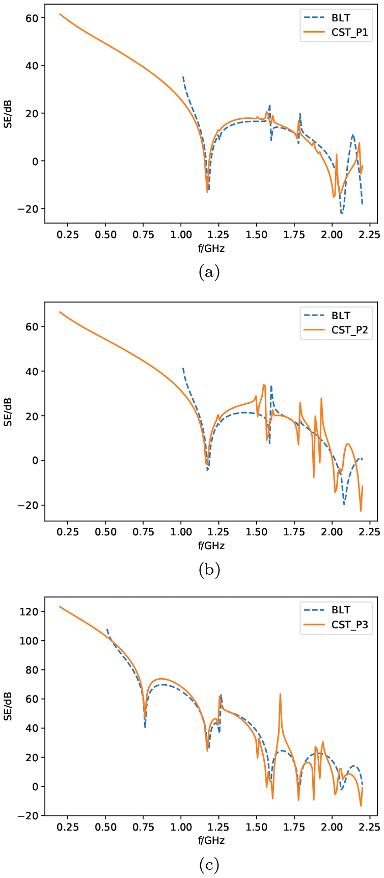
Figure 4: Comparison between the SE result from the BLT equation with that of CST for observe points 1, 2, and 3, respectively.

Figure 4(a) shows SE at $P_1$, and this is also the center of Enclosure 1. It can be observed that the result calculated by the proposed method is in good agreement with the simulation result of CST. The minimum SE values due to the resonance effect are just located at the resonance points which can be calculated by eqn (16):

$$f_{mnh}=\frac{C}{2}\sqrt{{\left(\frac{m}{a}\right)}^2+{\left(\frac{n}{b}\right)}^2+{\left(\frac{h}{d}\right)}^2}$$

(16)

where $m$, $n$, and $h$ are determined by the wave modes in the enclosure. In Enclosure 1, the resonant frequency is 1179.24 MHz for the $T{E}_{101}$ mode and 1600.78 MHz for the $T{E}_{102}$ mode. 1000 MHz is the cutoff frequency of $T{E}_{10}$ mode Enclosure 1, and the cutoff frequency of $T{E}_{30}$ in Enclosure 1 is 3000 MHz; consequently, the higher-order propagation modes are blocked.

Figure 4(b) shows the SE at $P_2$, which have a similar SE of $P_1$due to the same dimension size. The difference of SE results from the different dimensions of the apertures.

Figure 4(c) shows the SE at $P_3$, and compared with SE at the observation point $P_1$, the SE at the center of Enclosure 3 improves by 20 dB in most frequency ranges, except at the resonance points. From Figure 4(c), it can be seen that the result of SE with the proposed method is in good agreement with that of CST-MWS. Figure 4(c) shows the resonant frequencies of different transmission modes, such as 763.44 ($T{E}_{101}$), 1154.49 ($T{E}_{201}$), 1257.52 ($T{E}_{102}$), 1607.12 ($T{E}_{301}$), 1801.54 ($T{E}_{103}$), and 2081.54 MHz ($T{E}_{401}$). As we have seen in Section 2, $a{p}_3$ and $a{p}_4$are not at the center of the front wall of Enclosure 3, so $T{E}_{201}$and $T{E}_{401}$ modes appear in Enclosure 3; Note that the $T{E}_{201}$ mode is also $T{E}_{101}$ mode in Enclosure 1 and Enclosure 2, which further weakens the SE in Enclosure 3. We can conclude that the shielding capacity of the inner enclosures is obviously much better than that of the outer enclosure, and the resonant modes of the different enclosures influence each other through the apertures; this must be considered in practice. By observing eqn (16), we can also see that reducing the size of the enclosure will increase the resonant frequency; in other words, separating the outer enclosure into two smaller enclosures helps to improve the SE of the inner enclosure.

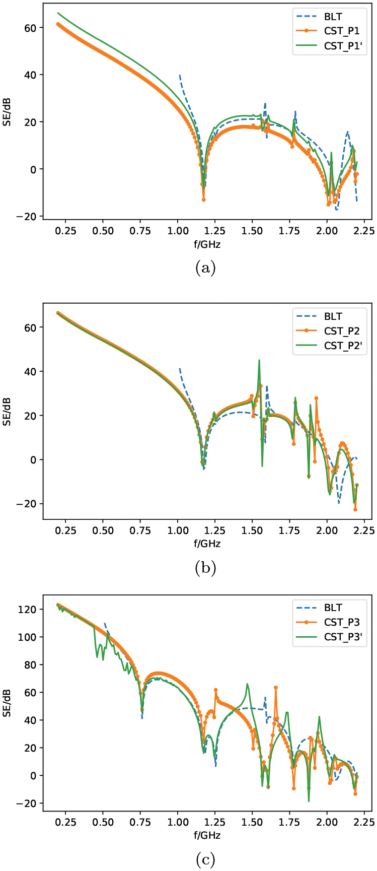
Figure 5: Comparison between the SE results from $P_1^{\prime }$, $P_2^{\prime }$, and $P_3^{\prime }$ with the same position and the original position $P_1$, $P_2$, and $P_3$ of CST.

B. Results of different positions

By applying the position factor in eqn (4), we obtain voltage distribution at any observation point: $v_p^{{}^{\prime }}=v_p{C}_a$; then an off-center observation point can be considered in this way. We have moved the observation points to new positions, and the new points $P_1^{\prime }$, $P_2^{\prime }$, and $P_3^{\prime }$are located in (30, 50, 380), (225, 80, 380), and (150, 50, 100).

Figure 5(a) shows the SE at $P_1^{\prime }$, and we can see that the SE at $P_1^{\prime }$ is about 5 dB higher than at $P_1$, indicating that the off-center point has a better SE.

Figure 5(b) shows the SE at $P_2^{\prime }$. Unlike the case of $P_1^{\prime }$, the SE of $P_2^{\prime }$ is very close to $P_2$. Since $T{E}_{10}$ is the main mode in Enclosure 2, it leads to a consistent voltage distribution in the $y$-axis direction.

Figure 5(c) shows the SE at $P_3^{\prime }$. We vary the $z$ coordinate by changing $d$ in the propagation matrix. It can be observed that the results of SE for the same enclosure differ greatly between two different monitor points.

All cases were calculated on the same computer running a 2.2-GHz Intel i7-8750 CPU. The CST takes 25–30 minutes for a simulation with 200 frequency points, while the fast algorithm takes no more than 0.2 seconds for the same case, indicating the high computational efficiency of the fast algorithm compared to the CST simulation.

IV. CONCLUSION

In this paper, we propose a fast algorithm based on EMT theory and the BLT equation to analyze the shielding performance of an apertured triple enclosure illuminated by an external plane wave. We derive a double three-port scattering matrix to describe the coupling relationship of the triple enclosure. By introducing the position factor $c_a$, the SE and resonances at any observation point can be easily predicted. Several observation points are presented to demonstrate the validity and accuracy of the algorithm. The proposed method has a good agreement with numerical method over a wide frequency range, while it can significantly improve the computation speed. This algorithm also proves that the BLT equation can handle complex enclosures by changing the EMT relationship.

REFERENCES

[1] T. Cvetković, V. Milutinović, N. Dončov, and B. Milovanović, “Numerical Investigation of Monitoring Antenna Influence on Shielding Effectiveness Characterization,” The Applied Computational Electromagnetics Society Journal (ACES), pp. 837-846, 2014.

[2] S. Georgakopoulos, C. Birtcher, and C. Balanis, “HIRF penetration through apertures: FDTD versus measurements,” IEEE Transactions on Electromagnetic Compatibility, vol. 43, no. 3, pp. 282-294, Aug. 2001.

[3] R. Araneo and G. Lovat, “Fast MoM Analysis of the Shielding Effectiveness of Rectangular Enclosures With Apertures, Metal Plates, and Conducting Objects,” IEEE Transactions on Electromagnetic Compatibility, vol. 51, no. 2, pp. 274-283, May 2009.

[4] B. Audone and M. Balma, “Shielding effectiveness of apertures in rectangular cavities,” IEEE Transactions on Electromagnetic Compatibility, vol. 31, no. 1, pp. 102-106, Feb. 1989.

[5] B.-L. Nie, P.-A. Du, Y.-T. Yu, and Z. Shi, “Study of the Shielding Properties of Enclosures With Apertures at Higher Frequencies Using the Transmission-Line Modeling Method,” IEEE Transactions on Electromagnetic Compatibility, vol. 53, no. 1, pp. 73-81, Feb. 2011.

[6] M. P. Robinson, T. M. Benson, C. Christopoulos, J. F. Dawson, M. D. Ganley, A. C. Marvin, S. J. Porter, and D. W. P. Thomas, “Analytical formulation for the shielding effectiveness of enclosures with apertures,” IEEE Transactions on Electromagnetic Compatibility, vol. 40, no. 3, p. 9, 1998.

[7] M. P. Robinson, J. D. Turner, D. W. P. Thomas, J. F. Dawson, M. D. Ganley, A. C. Marvin, S. J. Porter, T. M. Benson, and C. Christopoulos, “Shielding effectiveness of a rectangular enclosure with a rectangular aperture,” Electronics Letters, vol. 32, no. 17, pp. 1559-1560, Aug. 1996, publisher: IET Digital Library.

[8] F. Po’ad, M. Jenu, C. Christopoulos, and D. Thomas, “Analytical and experimental study of the shielding effectiveness of a metallic enclosure with off-centered apertures,” in 2006 17th International Zurich Symposium on Electromagnetic Compatibility, pp. 618-621, IEEE, Singapore, 2006.

[9] C.-C. Wang, C.-Q. Zhu, X. Zhou, and Z.-F. Gu, “Calculation and Analysis of Shielding Effectiveness of the Rectangular Enclosure with Apertures,” The Applied Computational Electromagnetics Society Journal (ACES), pp. 535-545, 2013.

[10] M.-C. Yin and P.-A. Du, “An Improved Circuit Model for the Prediction of the Shielding Effectiveness and Resonances of an Enclosure With Apertures,” IEEE Transactions on Electromagnetic Compatibility, vol. 58, no. 2, pp. 448-456, Apr. 2016.

[11] B.-L. Nie and P.-A. Du, “An Efficient and Reliable Circuit Model for the Shielding Effectiveness Prediction of an Enclosure With an Aperture,” IEEE Transactions on Electromagnetic Compatibility, vol. 57, no. 3, pp. 357-364, Jun. 2015.

[12] F. Tesche, “Topological concepts for internal EMP interaction,” IEEE Transactions on Antennas and Propagation, vol. 26, no. 1, pp. 60-64, Jan. 1978.

[13] C. E. Baum, “Electromagnetic Topology for the Analysis and Design of Complex Electromagnetic Systems,” in J. E. Thompson and L. H. Luessen, editors, Fast Electrical and Optical Measurements: Volume I — Current and Voltage Measurements/ Volume II — Optical Measurements, NATO ASI Series, pp. 467-547, Springer Netherlands, Dordrecht, 1986.

[14] F. M. Tesche, J. M. Keen, and C. M. Butler, “Example of the use of the BLT equation for EM field propagation and coupling calculations,” URSI Radio Science Bulletin, vol. 2005, no. 312, pp. 32-47, Mar. 2005.

[15] F. M. Tesche, “On the Analysis of a Transmission Line With Nonlinear Terminations Using the Time-Dependent BLT Equation,” IEEE Transactions on Electromagnetic Compatibility, vol. 49, no. 2, pp. 427-433, May 2007.

[16] Kan Yong, Yan Li-Ping, Zhao Xiang, Zhou Hai-Jing, Liu Qiang, and Huang Ka-Ma, “Electromagnetic topology based fast algorithm for shielding effectiveness estimation of multiple enclosures with apertures,” Acta Physica Sinica, vol. 65, no. 3, p. 030702, 2016.

[17] K. Gupta, R. Garg, I. Bahl, and P. Bhartia, Microstrip Lines and Slotlines, Artech House,1996.

BIOGRAPHIES

Jincheng Zhou was born in Jiangsu, China, in 1990. He received the B.A. degree from Xi’an Technological University, China, in 2008. He is currently working toward the Ph.D. degree with at the School of Information and Electronics, Beijing Institute of Technology. His research interests include radio propagation, EMC, and EM protection.

Xuetian Wang was born in Jiangsu, China, in 1961. He received the Ph.D. from the Department of Electronic Engineering, Beijing Institute of Technology in 2002. He has been working with t Beijing Institute of Technology as a Researcher since August 2001, and he has been a Professor since 2003. His research interests include EMC, EM protection, and electromagnetic radiation characteristics.

ACES JOURNAL, Vol. 37, No. 2, 246–252.
doi: 10.13052/2022.ACES.J.370214
© 2021 River Publishers

Abstract

I. INTRODUCTION

II. ELECTROMAGNETIC TOPOLOGICAL MODEL

III. RESULTS AND DISCUSSION

A. Results of different enclosures

B. Results of different positions

IV. CONCLUSION

REFERENCES

BIOGRAPHIES