Analytical Approximations for the Maximum-to-mean Ratio of the E-field in a Reverberation Chamber: A Review

Qian Xu¹, Rui Jia², Lifei Geng², Hao Guo², and Yongjiu Zhao¹

¹College of Electronic and Information Engineering, Nanjing University of Aeronautics and Astronautics, Nanjing, 211106, China
emxu@foxmail.com, yjzhao@nuaa.edu.cn

²State Key Laboratory of Complex Electromagnetic Environment Effects on Electronic and Information System, Luo Yang, China
jiarui315@163.com

Submitted On: December 17, 2021; Accepted On: August 18, 2022

Abstract

The expected value of the maximum value of the rectangular E-field is important in radiated susceptibility testing in a reverberation chamber. In this paper, different forms of equations for the maximum-to-mean ratio of the rectangular E-field are reviewed. Important derivations are summarized and detailed. It is interesting to note that some series which could be difficult to deal with from mathematics could be solved efficiently from physical point of view. The relationship between the independent sample number N and the parameters in generalized extreme value distribution is also given.

Index Terms: maximum-to-mean ratio, reverberation chamber, statistical electromagnetics.

1 INTRODUCTION

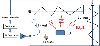
Reverberation Chambers (RCs) have been widely used in electromagnetic compatibility (EMC) testing [1]. Compared with an anechoic chamber, no radio absorber is used on the walls, thus a rich multipath environment can be created in an RC. By rotating the mechanical stirrers in an RC, statistically uniform and isotropic electromagnetic fields can be created. A typical measurement setup is illustrated in Fig. 1. For the radiated susceptibility testing in an RC, the maximum E-field is of interest [1], [2] as the device under test (DUT) could be malfunctioned by the maximum E-field.

In an RC, statistical electromagnetics are used to characterize the field properties. The probability density function (PDF) and the cumulative distribution function (CDF) of the maximum rectangular E-field have been given in [2]–[5]. Approximate analytical equations have also been given in [4], [5] for large independent sample number N. Different forms of equations exist, and the similarities and equivalencies among them have not been summarized.

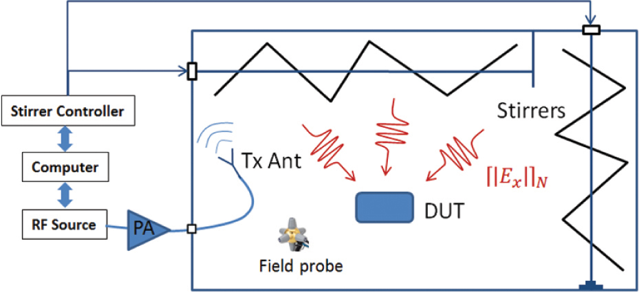
Figure 1: A schematic plot of radiated susceptibility in an RC.

In this paper, we review the analytical equations for the expected value and the standard deviation of the maximum E-fields in literatures. Numerical results are calculated and compared with different forms of analytical equations.

2 THEORY

The mean rectangular E-field strength in an RC is easy to estimate. However, the maximum rectangular E-field strength is of interest in many scenarios for EMC testing. The maximum-to-mean ratio of the rectangular E-field in an RC has been well studied in [2]–[5]. The PDF and the CDF of the maximum rectangular E-field in an RC are [2]–[5]:

$$p\left(x\right)=\frac{Nx}{{\sigma }^2}{\left[1-\exp \left(\frac{-x^2}{2{\sigma }^2}\right)\right]}^{N-1}\exp \mathit{\hspace{1em}}\left(\frac{-x^2}{2{\sigma }^2}\right),$$

(1)

and:

$$F\left(x\right)={\left[1-\exp \left(\frac{-x^2}{2{\sigma }^2}\right)\right]}^N,$$

(2)

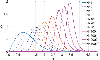
where N is the independent sample number, $x$ represents the maximum value of the rectangular E-field $x={\lceil \left|E_x\right|\rceil }_N$, and ${\lceil \cdot \rceil }_N$ represents the maximum value from N samples. The PDF of the normalized ${\lceil \left|E_x\right|\rceil }_N$ can be obtained by setting $\sigma =\sqrt{2/\pi }$, as the mean value of $\left|E_x\right|$ is $\sigma \sqrt{\pi /2}$. For different N, the PDF plots are illustrated in Fig. 2. It can be observed that when N increases, the expected value of the maximum E-field increases. The confidence interval of maximum E-field can be calculated from CDF in (2) [1], [5].

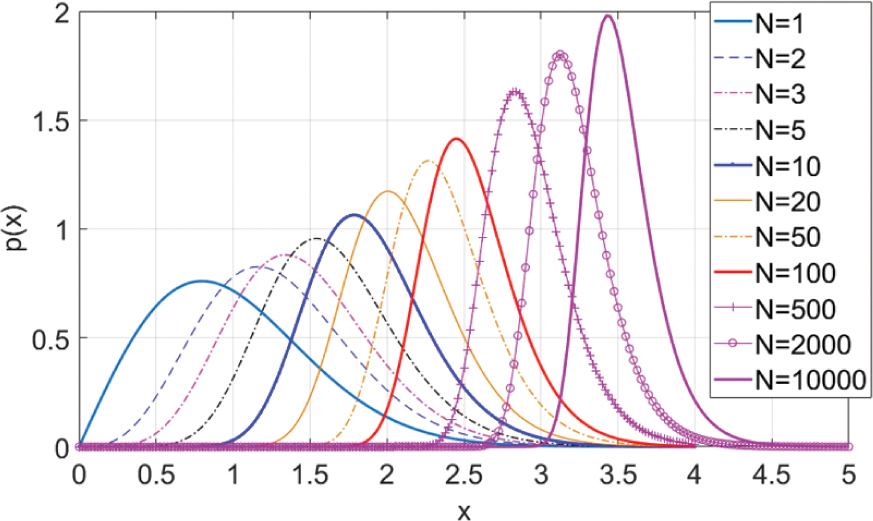
Figure 2: PDF plots of the normalized maximum E-field (normalized to the mean value $⟨\left|E_x\right|⟩$) for different independent sample number N.

The expected value of the maximum-to-mean ratio of the rectangular E-field be expressed as [2], [5]:

$\alpha \left(N\right)$	$={\displaystyle \frac{⟨{\lceil \left|E_x\right|\rceil }_N⟩}{⟨\left|E_x\right|⟩}}$
$={\displaystyle \frac{{\int }_0^{\mathrm{\infty }}N{x}^2{\left[1-\exp \left(\frac{-x^2}{2}\right)\right]}^{N-1}\exp \mathit{\hspace{1em}}\left(\frac{-x^2}{2}\right)dx}{\sqrt{\pi /2}}}.$	(3)

However, numerical integration is required to evaluate (3) using a computer, an approximate equation could be necessary to have a quick estimation for a given N. By applying the binomial theorem:

$\alpha \left(N\right)$
$=$	${\displaystyle \frac{{\int }_0^{\mathrm{\infty }}N{x}^2{\sum }_{k=0}^{N-1}\left(\genfrac{}{}{0pt}{}{N-1}{k}\right){\left[-\exp \left(\frac{-x^2}{2}\right)\right]}^k\exp \mathit{\hspace{1em}}\left(\frac{-x^2}{2}\right)dx}{\sqrt{\pi /2}}}$
$=$	${\displaystyle \frac{{\sum }_{k=0}^{N-1}N\left(\genfrac{}{}{0pt}{}{N-1}{k}\right){\left(-1\right)}^k{\int }_0^{\mathrm{\infty }}{x}^2{\left[\exp \left(\frac{-x^2}{2}\right)\right]}^{k+1}\mathit{d}x}{\sqrt{\pi /2}}}$
$=$	${\displaystyle \frac{{\sum }_{k=0}^{N-1}N\left(\genfrac{}{}{0pt}{}{N-1}{k}\right)\frac{{\left(-1\right)}^k\sqrt{\pi }}{\left(k+1\right)\sqrt{2k+2}}}{\sqrt{\pi /2}}}$
$=$	${\displaystyle \sum _{k=0}^{N-1}}{\displaystyle \frac{N!{\left(-1\right)}^k}{\left(N-k-1\right)!\left(k+1\right)!\sqrt{k+1}}}$
$=$	${\displaystyle \sum _{k=0}^{N-1}}s\left(k\right).$	(4)

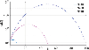
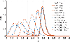
Although (3) is converted to the summation of a finite series, (4) is still not easy to evaluate. Symbolic calculation is required to maintain high precision, as the magnitude of $s\left(k\right)$ resonant drastically. A plot of $\left|s(k)\right|$ is illustrated in Fig. 3, as can be seen, when N is large, the magnitude of the series varies from 10$0^{}$ to 10${30}^{}$. If there is no special treatment for $s(k)$, numerical calculation is easy to diverge for large N and wrong results could be obtained.

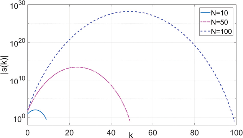
Figure 3: Plots of $s(k)$ for different N, symbolic calculation is used to keep precision.

It seems we cannot go further from (4). Instead, we can approach it physically. Suppose an E-field probe (the Rx antenna) is placed inside a well-stirred RC, it can be found that the maximum received power ($\max (P_{\mathrm{rRC}})={\lceil P_{\mathrm{rRC}}\rceil }_N$) can be expressed as [2]:

$$\sqrt{\max (P_{\mathrm{rRC}})}\approx \frac{\max \left(\left|E_x\right|\right)\lambda \sqrt{{\eta }_{\mathrm{Rx}}}}{8\pi \sqrt{5}},$$

(5)

where $\left|E_x\right|$ represents the tangential component of the E-field in an RC ($⟨{\left|E_x\right|}^2⟩=4{⟨\left|E_x\right|⟩}^2/\pi$, $\max \left(\left|E_x\right|\right)={\lceil \left|E_x\right|\rceil }_N$), $\lambda$ is the wavelength, and ${\eta }_{Rx}$ is the efficiency (including mismatch loss) of the Rx antenna respectively. It is interesting to compare it with received power in an anechoic chamber (AC):

$$\sqrt{P_{\mathrm{rAC}}}=\frac{E_{\mathrm{AC}}\lambda \sqrt{{\eta }_{\mathrm{Rx}}}}{8\pi \sqrt{5}}\sqrt{2D/3},$$

(6)

where $E_{\mathrm{AC}}$ is the magnitude of the incident E-field and $D$ is the directivity of the Rx antenna in the direction of the incident wave. Not surprisingly, $D$ plays an important role in an AC. it can be found that when $D=3/2$, (5) and (6) give the same results. This means that if the E-field probe is calibrated in an AC, only when the directivity of the E-field probe is 3/2 (electrically small dipole antenna), the measured E-field in an RC is statistically accurate. When the frequency is high, the E-field probe is no longer an electrically small antenna; the measured mean E-field in an RC using the free space antenna factor is no longer accurate and ${\eta }_{Rx}$ is actually the key parameter. This effect is well known in standards related to RC measurements [1]. At high frequencies, an antenna is normally used to monitor the E-fields inside an RC instead of using an E-field probe.

From statistical analysis in [2]:

$$\frac{\max \left(P_{\mathrm{rRC}}\right)}{⟨P_{\mathrm{rRC}}⟩}\approx \sum _{k=1}^N\frac{1}{k}.$$

(7)

Note that [2], [7]:

$⟨P_{\mathrm{rRC}}⟩$	$={\displaystyle \frac{1}{2}}{\displaystyle \frac{E_0^2}{\eta }}{\displaystyle \frac{{\lambda }^2}{4\pi }}{\eta }_{\mathrm{Rx}}={\displaystyle \frac{3}{2}}{\displaystyle \frac{⟨{\left|E_x\right|}^2⟩}{\eta }}{\displaystyle \frac{{\lambda }^2}{4\pi }}{\eta }_{\mathrm{Rx}}$
$={\displaystyle \frac{6{⟨\left|E_x\right|⟩}^2}{\pi \eta }}{\displaystyle \frac{{\lambda }^2}{4\pi }}{\eta }_{\mathrm{Rx}}.$	(8)

From (5), (7) and (8) we have:

$$\max \left(\left|E_x\right|\right)\approx \frac{8\pi \sqrt{5}}{\lambda \sqrt{{\eta }_{\mathrm{Rx}}}}\sqrt{\frac{6{⟨\left|E_x\right|⟩}^2}{\pi \eta }\frac{{\lambda }^2}{4\pi }{\eta }_{\mathrm{Rx}}\sum _{k=1}^N\frac{1}{k}}.$$

(9)

Thus for large N:

$$\alpha \left(N\right)\approx \frac{\max \left(\left|E_x\right|\right)}{⟨\left|E_x\right|⟩}\approx \sqrt{\frac{4}{\pi }\sum _{k=1}^N\frac{1}{k}}.$$

(10)

The problem is now converted to the partial sum of the harmonic series. The following equation can be used [8]:

$$\sum _{k=1}^N\frac{1}{k}=\gamma +{\psi }_0\left(N+1\right),$$

(11)

where $\gamma \approx$0.5772 is the Euler-Mascheroni constant, ${\psi }_0\left(x\right)$ is the digamma function:

${\psi }_0\left(N+1\right)$	$\approx \ln N+{\displaystyle \frac{1}{2N}}-{\displaystyle \sum _{n=1}^{\mathrm{\infty }}}{\displaystyle \frac{B_{2n}}{2n{N}^{2n}}}$
$=\ln N+{\displaystyle \frac{1}{2N}}-{\displaystyle \frac{1}{12N^2}}+{\displaystyle \frac{1}{120N^4}}-{\displaystyle \frac{1}{252N^6}}+\mathrm{\dots },$

and $B_{2n}$ is the Bernoulli number $\frac{x}{\left(e^x-1\right)}={\sum }_{n=0}^{\mathrm{\infty }}\frac{B_n{x}^n}{n!}$. Thus we have:

$$\alpha \left(N\right)\approx \sqrt{\frac{4}{\pi }\left(\gamma +\ln N+\frac{1}{2N}-\frac{1}{12N^2}+\frac{1}{120N^4}-\frac{1}{252N^6}+\mathrm{\dots }\right)}.$$

(12)

Now we have obtained an analytical approximation for (3). In [4], the CDF value of 0.5 is used to calculate the expected value:

$$\alpha \left(N\right)\approx \sqrt{\frac{4}{\pi }\ln \frac{1}{\left[1-{0.5}^{\frac{1}{N}}\right]}}.$$

(13)

In [1] and [5], a similar expression is given with $\alpha \left(N\right)\approx \sqrt{\frac{4}{\pi }\left[0.5772+\ln \left(N+1\right)-\frac{1}{2(N+1)}\right]}$with slightly different parameters. Another approximation is given in [8] for the partial sum of harmonic series

${\displaystyle \sum _{k=1}^N}{\displaystyle \frac{1}{k}}\approx \left(2N+1\right){\tan }^{-1}\left({\displaystyle \frac{1}{2N+1}}\right)$

$+{\displaystyle \frac{1}{2}}\ln \left({\displaystyle \frac{2N^2+2N+1}{2}}\right)$

$+{\displaystyle \frac{56N^6+168N^5+140N^4-42N^2-14N-1}{2520{\left(2N^2+2N+1\right)}^7}}$
$-{\displaystyle \frac{6N^2+6N+1}{180{\left(2N^2+2N+1\right)}^3}}+\gamma -1.$	(14)

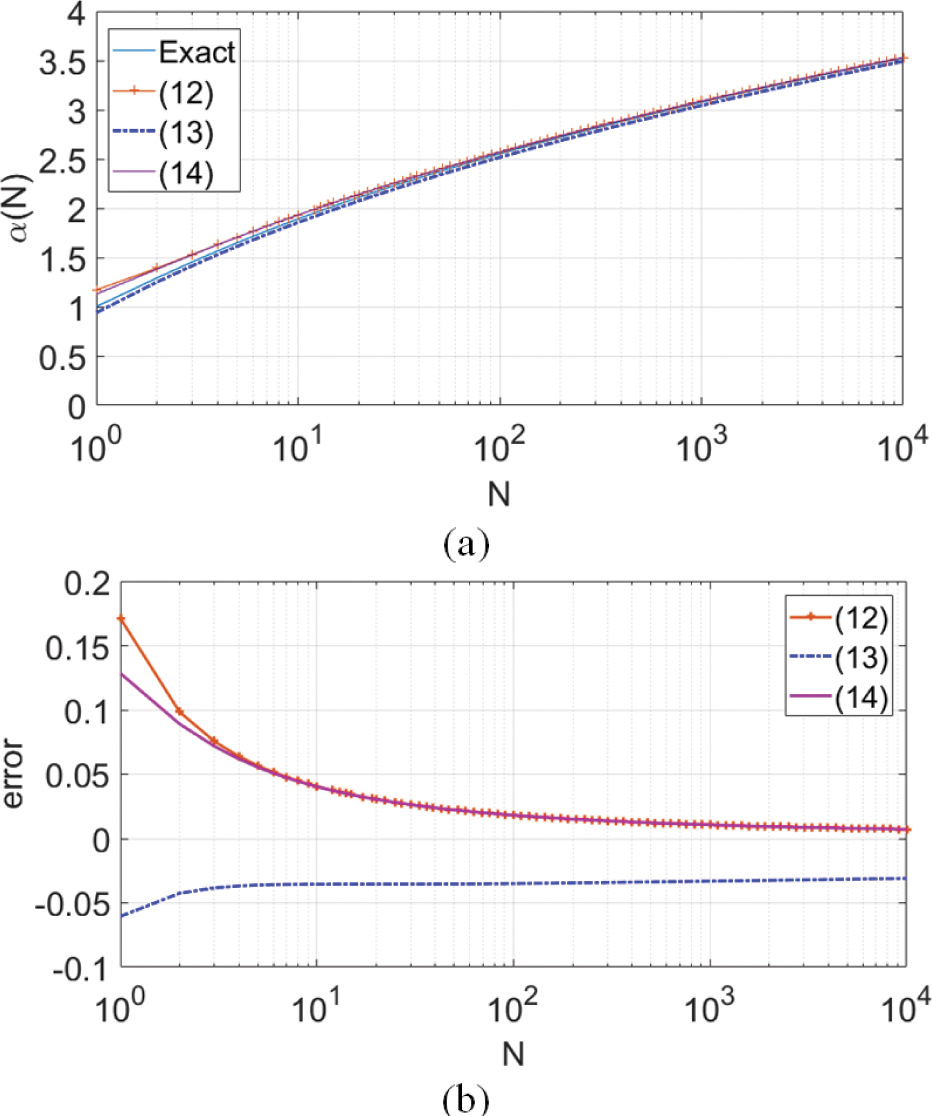
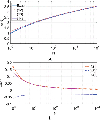
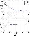
Figure 4: (a) Plots of (4), (12)-(14) for different N, (b) error plot of (12)-(14), units are in linear.

A comparison of $\alpha \left(N\right)$ is given in Fig. 4 (a) using (12)-(14), (12) is truncated with 3 terms, while the exact value is calculated using symbolic calculation in (4). The difference between (12)-(14) and the exact values (the error plots) are illustrated in Fig. 4 (b), respectively. As can be seen, (12) and (14) give smaller errors than (13). However, they all give good approximations when N is large.

For the approximate value of the relative standard deviation of ${\lceil \left|E_x\right|\rceil }_N$, we can start from the definition

${\mathrm{std}}_{\mathrm{rel}}\left({\lceil \left|E_x\right|\rceil }_N\right)$	$={\displaystyle \frac{\sqrt{{\int }_0^{\mathrm{\infty }}{x}^{2}p\left(x\right)\mathit{d}x-\frac{\pi }{2}\alpha {\left(N\right)}^2}}{\alpha \left(N\right)\sqrt{\frac{\pi }{2}}}}$
$=$	$\mathrm{}{\displaystyle \frac{\sqrt{{\sum }_{k=0}^{N-1}N\left(\genfrac{}{}{0pt}{}{N-1}{K}\right){(-1)}^k{\int }_0^{\mathrm{\infty }}{x}^3{\left[\exp \left(\frac{-x^2}{2}\right)\right]}^{k+1}\mathit{d}x-\alpha {\left(N\right)}^2}}{\alpha \left(N\right)\sqrt{\frac{\pi }{2}}}}$
$=$	${\displaystyle \frac{\sqrt{{\sum }_{k=0}^{N-1}\frac{N!{(-1)}^{k}2}{\left(N-k-1\right)!\left(k+1\right)!(k+1)}-\frac{\pi }{2}\alpha {\left(N\right)}^2}}{\alpha \left(N\right)\sqrt{\frac{\pi }{2}}}}$
$=$	${\displaystyle \frac{\sqrt{2{\sum }_{k=1}^N\frac{1}{k}-\frac{\pi }{2}\alpha {\left(N\right)}^2}}{\alpha \left(N\right)\sqrt{\frac{\pi }{2}}}}$
$=$	$\sqrt{{\displaystyle \frac{4}{\pi }}{\displaystyle \frac{{\sum }_{k=1}^N\frac{1}{k}}{\alpha {\left(N\right)}^2}}-1}.$	(15)

It seems we cannot go further from (15). To obtain the approximate value of (15), a different approach can be used [5]. We start from the relative standard deviation of ${\lceil {\left|E_x\right|}^2\rceil }_N$. From [2], we have:

${\mathrm{std}}_{\mathrm{rel}}({\lceil {\left|E_x\right|}^2\rceil }_N)$	$={\displaystyle \frac{\mathrm{std}({\lceil {\left|E_x\right|}^2\rceil }_N)}{⟨{\lceil {\left|E_x\right|}^2\rceil }_N⟩}}$
$=$	${\displaystyle \frac{\sqrt{{\sum }_{k=1}^N\frac{1}{k^2}}}{{\sum }_{k=1}^N\frac{1}{k}}},$	(16)

and we know that the uncertainty of power is 2 times the uncertainty of E-field (from $P\propto {\left|E_x\right|}^2$we have $dP/P\approx 2d\left|E_x\right|/\left|E_x\right|$) [5], thus the relative standard deviation of ${\lceil \left|E_x\right|\rceil }_N$ can be approximated as:

${\mathrm{std}}_{\mathrm{rel}}\left({\lceil \left|E_x\right|\rceil }_N\right)$	$\approx {\displaystyle \frac{1}{2}}{\mathrm{std}}_{\mathrm{rel}}\left({\lceil {\left|E_x\right|}^2\rceil }_N\right)\approx {\displaystyle \frac{1}{2}}{\displaystyle \frac{\sqrt{\frac{{\pi }^2}{6}-\frac{1}{N}}}{\gamma +{\psi }_0\left(N+1\right)}}$
$={\displaystyle \frac{1}{2}}{\displaystyle \frac{\sqrt{\frac{{\pi }^2}{6}-\frac{1}{N}}}{\gamma +\ln N+\frac{1}{2N}-\frac{1}{12N^2}+\mathrm{\dots }}},$	(17)

$$\approx \frac{\pi }{2\sqrt{6}}\frac{1}{\gamma +\ln N}.$$

(18)

In [5], a similar expression is given with $\frac{1}{2}\frac{\sqrt{\frac{{\pi }^2}{6}-\frac{N+1}{N(N+2)}}}{0.5772+\ln \left(N+1\right)-\frac{1}{2(N+1)}}$.

The plot of (15),(17) and (18) are illustrated in Fig. 5 (a), (15) is used as the reference values (the exact values), and the difference between (17), (18) and (15) are presented in Fig. 5 (b), respectively. It is interesting to note that the convergence speed of (18) is different from the mean value (by using the central limit theorem) which is $\frac{1}{\sqrt{N}}$ [5].

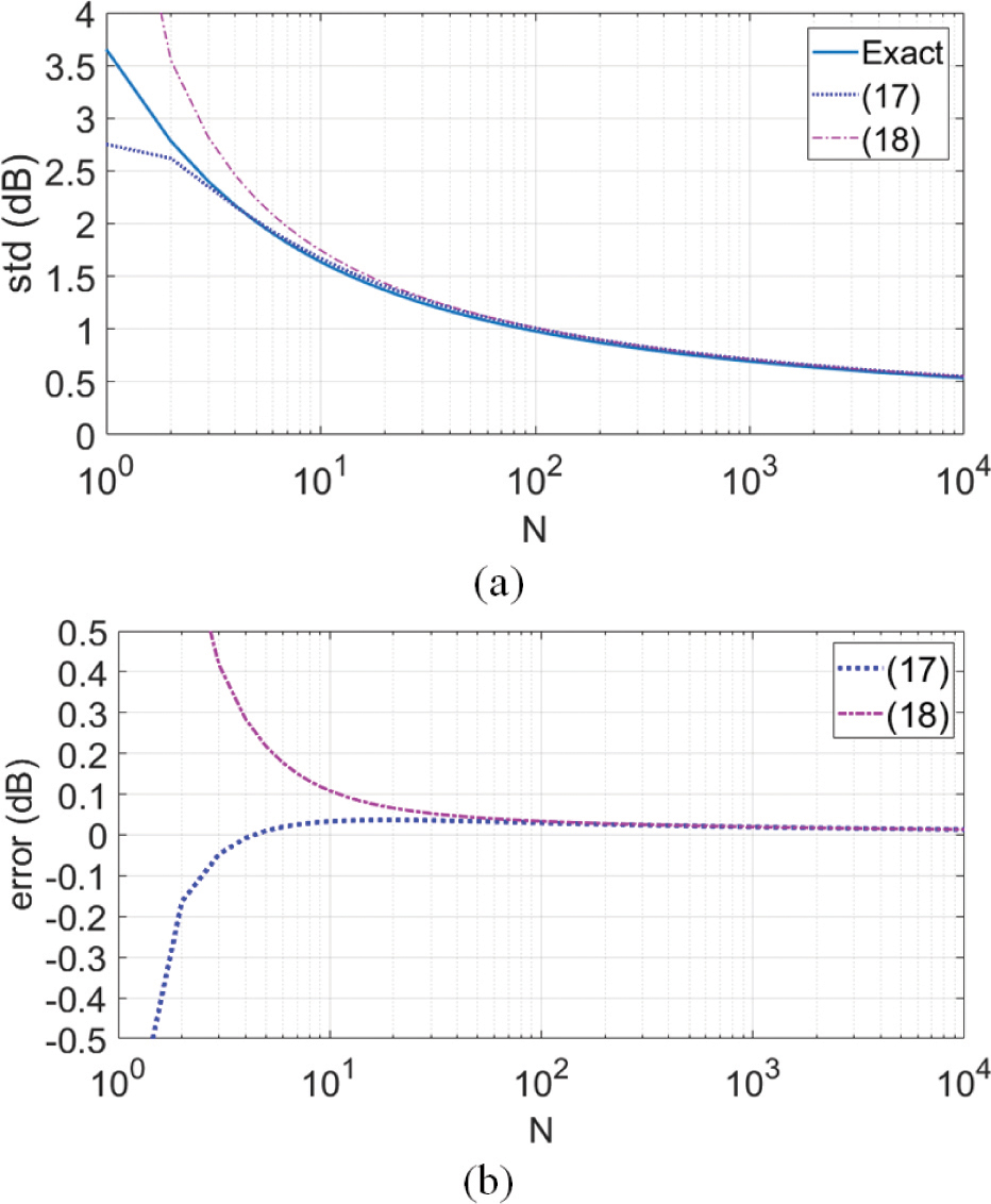
Figure 5: (a) Plots of the approximated relative standard deviation in dB units ($20\mathrm{l}\mathrm{o}\mathrm{g}10(1+{\mathrm{std}}_{\mathrm{rel}})$), (b) error plot of (17), (18), units are in dB.

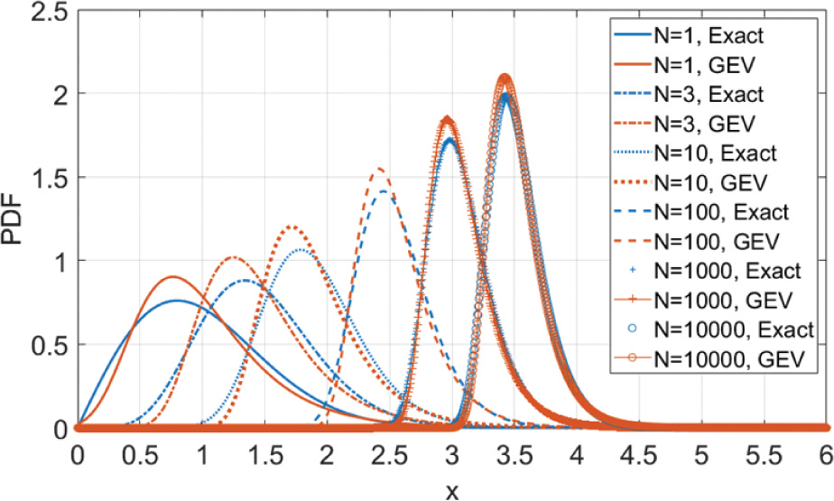
Figure 6: Comparison plots of exact PDFs and GEV PDFs for different N.

We can also link the parameters to the generalized extreme value distribution (GEV) [10]–[18] when $N\to \mathrm{\infty }$. By applying [10]:

$$s=\frac{\sqrt{6}}{\pi }\mathrm{std}=\frac{\sqrt{6}}{\pi }{\mathrm{std}}_{\mathrm{rel}}\left({\lceil \left|E_x\right|\rceil }_N\right)\alpha \left(N\right),$$

(19)

$$m=\alpha \left(N\right)-\gamma s.$$

(20)

The approximated GEV CDF is:

$$G_{\mathrm{GEV}}(x)=\exp \left[-\exp \left(-\frac{x-m}{s}\right)\right],$$

(21)

Table 1: A summary of maximum-to-mean ratio expressions

the PDF is:

$$p_{\mathrm{GEV}}(x)=\frac{1}{s}\exp \left[\frac{m-x-s\exp (-\frac{x-m}{s})}{s}\right]$$

(22)

When $N\to \mathrm{\infty }$, (19) and (20) can be approximated as:

$$s=\frac{\sqrt{6}}{\pi }\mathrm{std}\approx \frac{1}{\sqrt{\pi }\sqrt{\gamma +\ln N+\frac{1}{2N}}},$$

(23)

$$m\approx \sqrt{\frac{4}{\pi }\left(\gamma +\ln N+\frac{1}{2N}\right)}-\frac{\gamma }{\sqrt{\pi }\sqrt{\gamma +\ln N+\frac{1}{2N}}}.$$

(24)

The plot for the exact PDFs (1) and GEV PDFs (22) of the normalized maximum rectangular E-field are given in Fig. 6. As expected, when $N\to \mathrm{\infty }$, two PDFs are close to each other.

For the PDF of the maximum-to-mean ratio of the received power ${\lceil {\left|E_x\right|}^2\rceil }_N$, we have the same $p_{\mathrm{GEV}}(x)$ when $N\to \mathrm{\infty }$. The only difference is: the standard deviation and the expected value ($\alpha \left(N\right)$) in (19) and (20) are replaced by the values of $\sqrt{{\sum }_{k=1}^N{k}^{-2}}$ and ${\sum }_{k=1}^N{k}^{-1}$, respectively.

3 CONCLUSIONS

We have reviewed different analytical equations for the expected value and the standard deviation of the normalized maximum rectangular E-field in a well-stirred RC. Useful derivations are revisited and similar results are obtained. Numerical results show that: for small independent sample number N, we can calculate the results using the finite series directly; when $N>5$, very good approximations can be obtained for both the expected value and the standard deviation. Table 1 summarizes the expressions in different forms. The approximated analytical expressions are also linked to the parameters of the GEV parameters when $N\to \mathrm{\infty }$.

ACKNOWLEDGMENT

This work was supported in part by the Fund of Prospective Layout of Scientific Research for NUAA (Nanjing University of Aeronautics and Astronautics).

REFERENCES

[1] IEC 61000-4-21, Electromagnetic compatibility (EMC) – Part 4-21: Testing and measurement techniques – Reverberation chamber test methods, IEC Standard, Ed 2.0, 2011-01.

[2] J. Ladbury, G. Koepke, and D. Camell, Evaluation of the NASA Langley Research Center mode-stirred chamber facility, National Institute of Standards and Technology, Gaithersburg, MD, USA, Tech. Note 1508, Jan. 1999.

[3] T. H. Lehman and G. J. Freyer, “Characterization of the maximum test level in a reverberation chamber,” IEEE International Symposium on Electromagnetic Compatibility, pp. 44-47, 1997.

[4] L. R. Arnuat and P. D. West, Electric Field Probe Measurements in the NPL Untuned Stadium Reverberation Chamber, NPL CETM13, Sep. 1999.

[5] L. R. Arnaut, Measurement Uncertainty in Reverberation Chambers – I. Sample Statistics, NPL Report TQE 2, Dec. 2008.

[6] Q. Xu and Y. Huang, Anechoic and Reverberation Chambers: Theory, Design and Measurements, Wiley-IEEE, 2019.

[7] D. A. Hill, Electromagnetic Fields in Cavities: Deterministic and Statistical Theories, Hoboken, NJ, USA, Wiley, 2009.

[8] E. W. Weisstein, Harmonic Series, From MathWorld – A Wolfram Web Resource. https://mathworld.wolfram.com/HarmonicSeries.Html

[9] T. N. Vu, A New Approximation Formula for Computing the N-th Harmonic Number (Update), from Series Math Study Resource. http://www.seriesmathstudy.com/sms/ApproximateFormulaHarmonicNum, 11/11/2011.

[10] G. Gradoni and L. R. Arnaut, “Generalized extreme-value distributions of power near a boundary inside electromagnetic reverberation chambers,” IEEE Transactions on Electromagnetic Compatibility, vol. 52, no. 3, pp. 506-515, Aug. 2010.

[11] G. Orjubin, “Maximum field inside a reverberation chamber modeled by the generalized extreme value distribution,” IEEE Transactions on Electromagnetic Compatibility, vol. 49, no. 1, pp. 104-113, Feb. 2007.

[12] C. E. Hager and J. D. Rison, “On applying the generalized extreme value distribution to undermoded cavities within a reverberation chamber,” IEEE International Symposium on Electromagnetic Compatibility & Signal/Power Integrity (EMCSI), pp. 681-686, 2017.

[13] N. Nourshamsi, J. C. West, and C. F. Bunting, “Effects of aperture dimension on maximum field level inside nested chambers by applying the generalized extreme value distribution,” IEEE Symposium on Electromagnetic Compatibility, Signal Integrity and Power Integrity (EMC, SI & PI), pp. 628-633, 2018.

[14] N. Nourshamsi, J. C. West, and C. F. Bunting, “Investigation of electromagnetic complex cavities by applying the generalized extreme value distribution,” IEEE Symposium on Electromagnetic Compatibility, Signal Integrity and Power Integrity (EMC, SI & PI), pp. 622-627,2018.

[15] N. Nourshamsi, J. C. West, C. E. Hager, and C. F. Bunting, “Generalized extreme value distributions of fields in nested electromagnetic cavities,” IEEE Transactions on Electromagnetic Compatibility, vol. 61, no. 4, pp. 1337-1344, Aug.2019.

[16] P. Hu, Z. Zhou, X. Zhou, J. Li, J. Ji, M. Sheng, and P. Li, “Generalized extreme value distribution based framework for shielding effectiveness evaluation of undermoded enclosures,” International Symposium on Electromagnetic Compatibility-EMC EUROPE, pp. 1-6,2020.

[17] P. Hu, X. Zhou, and Z. Zhou, “On the modelling of maximum field distribution within reverberation chamber using the generalized extreme value theory,” IEEE MTT-S International Conference on Numerical Electromagnetic and Multiphysics Modeling and Optimization (NEMO), pp. 1-4, 2020.

[18] P. Hu, Z. Zhou, X. Zhou, and M. Sheng, “Maximum field strength within reverberation chamber: A comparison study,” 6th Global Electromagnetic Compatibility Conference (GEMCCON), pp. 1-4, 2020.

BIOGRAPHIES

Qian Xub (Member, IEEE) received the B.Eng. and M.Eng. degrees from the Department of Electronics and Information, Northwestern Polytechnical University, Xi’an, China, in 2007 and 2010, and received the PhD degree in electrical engineering from the University of Liverpool, U.K, in 2016. He is currently an Associate Professor at the College of Electronic and Information Engineering, Nanjing University of Aeronautics and Astronautics, China.

He was as a RF engineer in Nanjing, China in 2011, an Application Engineer at CST Company, Shanghai, China in 2012. His work at University of Liverpool was sponsored by Rainford EMC Systems Ltd. (now part of Microwave Vision Group) and Centre for Global Eco-Innovation. He has designed many chambers for the industry and has authored the book Anechoic and Reverberation Chambers: Theory, Design, and Measurements(Wiley-IEEE, 2019). His research interests include statistical electromagnetics, reverberation chamber, EMC and over-the-air testing.

Rui Jia received the B.Eng. degrees from the Department of Electronics and Information, Zhengzhou University, Zhengzhou, China, in 2008, and received the M.Eng. and Ph.D. degrees in electronic engineering from Mechanical Engineering College, Shijiazhuang, China, in 2010 and 2014, respectively. His research interests include statistical electromagnetics, reverberation chamber, and EMC.

Lifei Geng received the B.Eng., M.Eng. and Ph.D. degrees from the Department of Electronics and Information, Mechanical Engineering College, Shijiazhuang, China, in 2006, 2008 and 2013, respectively. His research interests include electromagnetic theory, reverberation chamber, and EMC.

Hao Guo received the B.Sc. and M.Sc. degrees from the Department of Physics, Dalian University of Technology, Dalian, China, in 2004, and 2009, respectively. His research interests include plasma, reverberation chamber, and EMC.

Yongjiu Zhao received the M.Eng. and Ph.D. degrees in electronic engineering from Xidian University, Xi’an, China, in 1990 and 1998, respectively. Since March 1990, he has been with the Department of Mechano-Electronic Engineering, Xidian University where he was a professor in 2004. From December 1999 to August 2000, he was a Research Associate with the Department of Electronic Engineering, The Chinese University of Hong Kong. His research interests include antenna design, microwave filter design and electromagnetic theory.

ACES JOURNAL, Vol. 37, No. 8, 842–847.
doi: 10.13052/2022.ACES.J.370802
© 2022 River Publishers

Abstract

1 INTRODUCTION

2 THEORY

3 CONCLUSIONS

ACKNOWLEDGMENT

REFERENCES

BIOGRAPHIES