A Brief History of Finite Element Method and Its Applications to Computational Electromagnetics

Stefano Selleri

Department of Information Engineering
University of Florence, Florence I-50139, Italy
stefano.selleri@unifi.it

Submitted On: December 29, 2021; Accepted On: May 2, 2022

Abstract

The development of the finite element method is traced, from its deepest roots, reaching back to the birth of calculus of variations in the 17th century, to its earliest steps, in parallel with the advent of computers, up to its applications in electromagnetics and its flourishing as one of the most versatile numerical methods in the field. A survey on papers published on finite elements, and on ACES Journal in particular, is also included.

Index Terms: Finite elements, history of computation, numerical methods.

I. THE PRODROMES

If, by finite elements (FEs), we intend the piecewise polynomial approximation of the solution of a partial differential equation (PDE) with adequate boundary conditions, then an exact date of its birth is known: January 1943. In an appendix to [1], Richard Courant (Figure 1), who had already investigated finite differences (FDs) in 1928 [2], sketched in two pages the essence of FE as intended above [3].

The paper was the written record of a dissertation on the equilibrium and vibrations of 2D domains: plates, membranes, and the like. The dissertation was held on May 3, 1941, and submitted as a paper on June 16, 1942. The matter treated in the appendix, the numerical solution of the problem, was indeed not included in the dissertation.

While Courant founded the computational part of FE, its essence was in the variational problem he was addressing, and variational problems are much older than FE.

Figure 1: Left to right: Richard Courant (1888-1972), John H. Argyris (1913-2004), and Ray W. Clough (1920-2016).

Johan Bernoulli in 1696 proposed the problem of the shortest time path connecting two points at different altitudes A and B [4]. This was something Galileo Galilei had already investigated, showing, experimentally, that a straight path is slower than an arc of circumference, but there was no proof that, in this latter, time was minimum [5].

Indeed, Isaac Newton, Jakob Bernoulli, Gottfried Wilhelm von Leibnitz, Ehrenfried Walter von Tschirnhaus, and Guillaume de l’Hôpital provided their own solution. In particular, Leibnitz exploited a piecewise linear approximation, which was a first step in his development of differential calculus, which he finally published [6], independently and shortly before Newton [7]. The question on the priority of this development lasted for decades. Leonhard Euler later worked on these kinds of problems and developed a brand-new branch of mathematics: the Calculus of Variations, a name suggested to Euler by Joseph-Louis Lagrange.

Indeed, also the idea of approximating a 2D variational problem on a mesh of triangles is older than Courant. Karl H. Schellbach in 1851 proposed a FE-like solution for determining the surface S of minimum area enclosed by a given curve by using a piecewise approximation of S on triangles [8].

A subsequent, important, step was done by John W. Strutt, Lord Rayleigh, who proposed a variational approach to the solution of PDEs with appropriate boundary conditions, which is of boundary value problems (BVPs) [9]. This approach was later developed by Walther Ritz, who conceived an approximation of the BVP solution as a finite linear combination of continuous functions [10]. One classical approach to FEs is indeed called Rayleigh–Ritz method.

An alternative approach to FE is that based on the idea of the minimization of an error defined in terms of an orthogonality condition versus some appropriate finite-dimensional sub-space. This technique was first suggested by Boris G. Galerkin [11] and developed by Alessandro Faedo [12], to what is now called a Faedo–Galerkin approach to FEs.

Before Courant, an FEs harbinger is the tear method introduced by Gabriel Kron, where a large and complex system is reduced to a network of interconnected small and simpler systems (1939). This was not indeed a solution of a PDE since the simple systems, the elements, were exactly specified, and, hence, the issue was just the algebraic interconnection [13]. Later, in 1941, Alexander Hrennikoff solved plane elasticity problems by splitting up the domain into little finite pieces whose stiffness was approximated by ideal bars, beams, and springs [14]. Shortly later, Douglas McHenry exploited a similar lattice analysis [15], leading to solutions which were primitive in mathematical and physical terms, but which were clearly leading to something implying a piecewise linear approximation over square or cubic cells.

John H. Argyris (Figure 1) then began in the 1950s to put all these ideas together by developing further Kron’s technique and adding an approximation which was truly based on a variational method [16]. In the same years, Samuel Levy introduced an evolution of Hrennikoff and McHenry lattice models by analyzing the behavior of aircraft wings via an assembly of box-elements comprising beams, torsion bars, rods, and shear panels [17]. Levy’s direct stiffness method had a great impact on aircraft structure analysis.

Actually, it is interesting to note that, after the early mathematical developments, the main actors on FEs in the 1950s and 1960s were not mathematicians but engineers, concerned more with design issues of airplanes than on the theoretical aspects of the method.

II. EARLY FINITE ELEMENTS

The first work truly embodying the essence of FEs and which can be pointed to as giving birth to the method is that of M. Jon Turner and co-workers [18]. In this paper, an attempt to exploit both a local approximation of the PDE of elasticity and an assembly strategy among local approximations was carried out, even if no variational principle was used. This paper was followed by the one by Ray W. Clough (Figure 1) where the name FE method finally appeared [19].

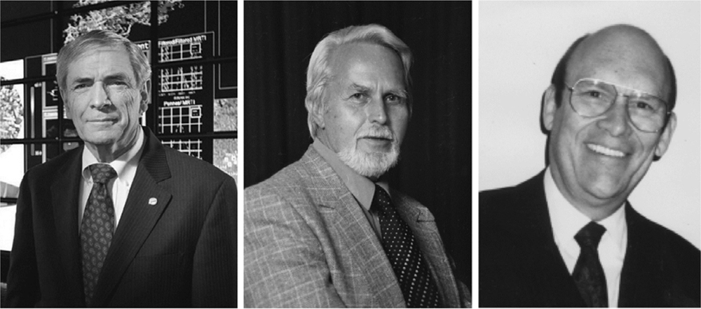
Figure 2: Left to right: J. Tinsley Oden (1936-), Olgierd C. Zienkiewicz (1921-2009), and Peter P. Silvester (1935-1996).

In the 1960s, the engineering community started to recognize the usefulness of FEs in its variational formulation, which is that of Rayleigh and Ritz, which, indeed, was applicable only to symmetric operators. In these years, aeronautics was the main application, and the Dayton Conferences on FEs held in 1965, 1968, and 1970 were occasions of remarkable and innovative accomplishments. In these same years, the fact that FEs could also be applied to unsymmetric operators become clear, with the solution of Navier–Stokes equations by J. Tinsen Oden (Figure 2) [20–22].

The first comprehensive textbook on FEs appeared in those same years, authored by Olgierd C. Zienkiewicz (Figure 2) and Yau K. Cheung in 1967 [23], shortly followed by one by Zienkiewicz alone [24].

Of course, these developments were made possible by the parallel development of digital computers, born around World War II, and of adequate programming languages, like FORTRAN introduced in 1954.

In the late 1960s, FEs were ported to wave electromagnetics by Peter P. Silvester (Figure 2) [25, 26] and, about a decade later, the first FEs book devoted to electrical engineers was published [27]. This is still, in its third edition, the bible of FEs for electrical engineers.

While practice was going fast, theory lagged. The first proof of convergence of FEs might be traced to Feng Kang [28], but the paper, being in Chinese, was overlooked. A second paper focused on a rigorous proof of convergence was published by M.W. Johnson and Richard W. McLay in 1968 [29]. Even if these are the first example of a rigorous theoretical approach to FEs, the tools we are now familiar with are a little older; simply, they were not explicitly applied.

Distribution theory, which indeed is at the basis of FE theory, was developed by Sergej L. Sobolev in 1936, when he introduced generalized functions to work with weak solutions of PDEs [30]. Later, Laurent Schwartz, in the 1940s, put together a sound theory of distributions [31, 32].

PDE theory and approximation theory in the mathematical world remained separate from variational methods and, hence, from FE application up to the late 1960s, when FE methodology and the theory of PDE approximation via functional analysis finally unite.

Then, in the 1970s, a great leap forward was done in the mathematical background of FEs: a-priori error estimator came out, elliptic linear problems were fully known, while parabolic and hyperbolic problems, also non-linear, were at their beginning in the FEs’ world.

Element interpolation characteristics were studied by Milo $\overset{ˇ}{s}$ Zl $\overset{´}{a}$ mal [33] followed by a fundamental comprehensive work by Ivo M. Babu $\overset{ˇ}{s}$ ka and A. Kadir Aziz [34], where Sobolev spaces and elliptic problems are comprehensively treated in an FE framework.

III. ELECTROMAGNETICS

Early applications to wave electromagnetics, developed after [25], tried to handle the vector nature of the fields by treating them component-by-component. Unfortunately, all these early vectorial methods were plagued by the occurrence of spurious modes, which are solutions of the numerical FEM problem which were non-physical [35].

An early analysis of spurious modes, which indeed were present also in FDs [36], can be found in Adalbert Konrad’s Ph.D. thesis [37] and in his paper where he first solves the vector curl–curl equation [38]. His analysis suggested that spurious modes were solutions, where the energy norm on the domain vanishes, but boundary conditions are not satisfied, and this was due to a lack of solenoidality of the FEM procedure.

Subsequent efforts on enforcing the vanishing of $\nabla \cdot B$ removed part of the spurious modes. Much research was done in this area by applying a penalty parameter effectively pushing spurious modes eigenvalues out of the range of interest yet having negligible effect on physical modes [39]. The issue on selecting the right value for the penalty parameter was addressed in [40]; yet, it was finally proven [41] that the curl–curl scheme inevitably led to spurious modes difficult to handle even with penalty scheme, while Helmholtz equation has spurious modes too, but these were ruled out by enforcing physical boundary conditions.

Jon P. Webb and Konrad applied a different approach based on an a-posteriori imposition of a set of constraints on the equation to guarantee solenoidality [42, 43]; however, this approach did not provegeneral.

In the same years, the concept of edge elements was developed by Jean-Claude Nedelec and others [44–48]. Edge elements do not over-constrain continuity of the field at element nodes but just enforce the physical continuity of the tangential field component at the edges, easily handling dielectric interfaces. Yet, these edge elements’ origin can be traced back to an FE unrelated work by Hassler Whitney few decades older [49].

These elements finally lead to a more accurate representation of the field in terms of element bases, getting rid of the spurious modes which had plagued the method in the beginning [50].

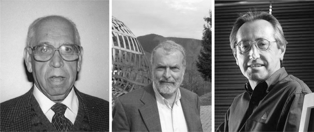
Figure 3: Left to right: A. Kadir Aziz (1923-2016), Jean-Claude Nedelec (1943- ), and Zoltan Cendes (1946- ).

Current state-of-the-art elements not only exclude spurious modes [51] but also allow to consider the divergent behavior of the electromagnetic field at edges and tips [52, 53].

Another key point in FE development in the 1970s and 1980s was handling unbounded radiation problems, FE being of course applicable only on domains of finite extension. Two lines of development emerged. In the first, the description of the field outside the finite domain was done in terms of a modal expansion (unimoment method [54], transfinite element method [55], and by moment method [56]) or in terms of an integral representation (FEs/boundary integral [57], FEs/method of moments [58], and field-feedback formulation [59]), but these were plagued by non-physical solutions too, that is, interior resonances [60]. Furthermore, these conditions, called exact were of global nature and spoiled the sparsity of the solving matrix. In the second line, local conditions – hence not spoiling sparsity – were enforced on the boundary assuming a far-field behavior. These so-called absorbing boundary conditions (ABC) are approximate, due to the far field assumption, and must be placed at a distance from the scatterer to have good accuracy; yet, they rapidly gained popularity either in 2D [61] or in 3D [62]. Another approach, in this contest, is that of adding a layer of absorbing material, either realistic [63] or fictitious and, hence, only numerical [64]. This latter, the so-called perfectly matched layer (PML) gained the greatest popularity in the end. Some wider insight on these developments can also be found in [65].

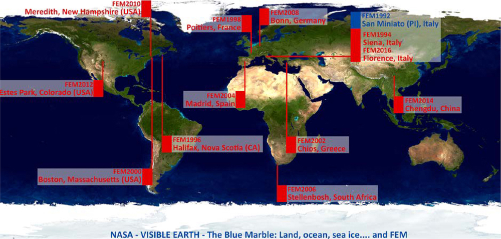
Figure 4: Location of the 13 FEM workshops for microwave engineering editions.

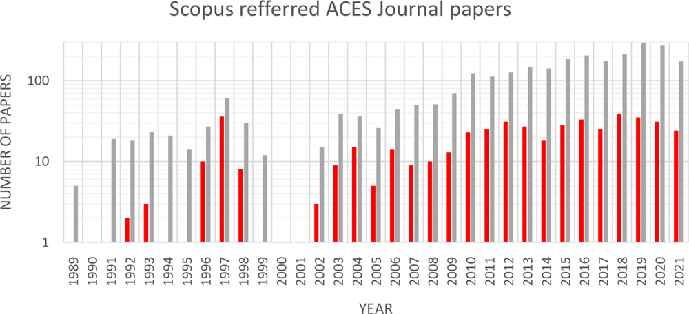
Figure 5: Finite elements (red bars) and total papers (gray bars) per year published on ACES Journal and referred in Scopus.

IV. MATURITY

By 1980, even if FEs have reached a good maturity in mechanical and civil engineering and in electromagnetics was still struggling with spurious modes, several “general purpose” codes began to be available to the engineers to treat broad classes of linear and nonlinear problems.

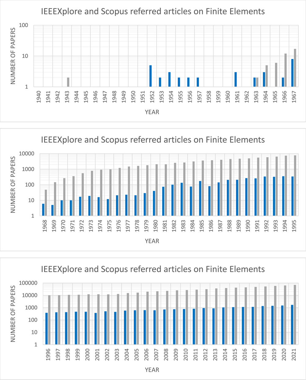
Figure 6: Finite elements papers per year referred on IEEExplore (blue bars) and on Scopus (gray bars) per year.

DYNA3D, originally developed by John O. Hallquist at Lawrence Liver more National Laboratory (LLNL), started in 1976 and became commercial in the 1980s.

ANSYS (ANalysis SYStems) ported its punched-card codes to Apple II in 1980, allowing for a first true graphical interface.

FEMAP was born in 1985 as a pre- and post-processor for one of the oldest codes, NASTRAN (NASa STRucture ANalysis). NASTRAN itself was developed by CSC and released to NASA in 1968. In 2001, NASA made the code publicly available.

StressCheck, released in 1989, was one of the first commercially available products to utilize the p-version of the FEs for structural analysis. P-version implies the possibly local increase of the order of the polynomial FE bases within an element to achieve higher accuracy, and is opposed to h-method, where the order of the bases is fixed and higher accuracy is achieved by refining the mesh into smaller elements.

In electromagnetism, Zoltan and Nicholas Cendes (Figure 3) founded Ansoft in 1984, marketing HFSS (high frequency structure simulator). Ansoft, after a long partnership with Hewlett-Packard, was finally acquired by ANSYS in 2008. HFSS is currently the standard, de facto, in FE analysis for electromagneticwaves.

Modern software package, on the other hand, comprises many different solvers to provide the users with maximum flexibility and multiphysics capabilities; so, nowadays, most of the EM simulation suites do include also FEs, as it is the case for CST, FEKO, COMSOL, etc.

Finally, for electromagnetics, and for wave electromagnetics, I wish to remember the biannual workshop, fully dedicated to FEs for Microwave Engineering which originated by a collaboration between the University of Florence, Italy and McGill University of Montreal, Canada, where P.P. Silvester was a professor. The workshop totaled 13 editions, the last independent one being in Florence in 2016 (Figure 4). A full history of these workshops can be found in [66, 67], while a deeper insight in the history of FEs in general can be found in [68].

V. ACES JOURNAL

It is interesting to analyze the presence of FE in scientific literature and on ACES Journal in particular. The Scopus database offers the possibility of advanced searches [69]. By limiting the search to ACES Journal (ISSN1054-4887), the total number of papers referred in Scopus per year can be obtained and, by further limiting the search to the paper containing the keyword “Finite Element*” in any field, the number of papers specifically dealing with FE is produced.

The result of these queries is sketched in Figure 5, showing in gray the total number of ACES papers indexed per year, starting from the first year where a paper on FE appeared (1989, just a single paper) up to 2021. While Scopus archives are apparently incomplete, since they index no paper at all in some years (1990 and 2000), they nevertheless provide an interesting insight: in the last 20 years, the number of FE papers was never below 10% of the total published ACES papers, with an average of 19% and a peak of 42% in 2004. Graphs are on logarithmic vertical scale to better appreciate the number of papers when they are few.

As a comparison, Figure 6 reports a similar query with the keyword “Finite Element*” in any field on the whole Scopus database and on IEEEXplore; results are limited to journal papers, again in logarithmic scale. Up to 1965, the presence of FE papers was sporadic; from 1966 to 2000, there was a steady increase, and from 2001 onwards, the increase was still present but less dramatic. This is well in accordance with what was stated earlier about the reach of maturity at the beginning of our century. Figure 6 is currently used on a Ph.D. course on FEs held both at the University of Florence and the Politecnico di Milano [70] and is derived from original bibliographical research in [71]. Small discrepancies with [71] are due to the different database used and their ever-going updates.

VI. CONCLUSION

A brief history of FE has been sketched, with a focus on its earliest, pioneeristic developments, followed by a bibliographical analysis on the number of FE papers in open literature in general on IEEE journals and on ACES Journal in particular. The latter, being committed to computational electromagnetics, hosted in this last 20 years a remarkable number of papers dealing with FEs and its applications.

ACKNOWLEDGMENTS

The author wishes to thank Prof. G. Pelosi, University of Florence, for the useful discussions provided in preparing this paper.

REFERENCES

[1] R. Courant, “Variational methods for the solution of problems of equilibrium and vibrations,” Bull. Amer. Math. Soc., vol. 49, no. 1, pp. 1-23,1943.

[2] R. Courant, K. O. Friedrichs, and H. Lewy, “Über die partiellen differenzengleichungen der mathematischenphysic [About the partial difference equations of the mathematical physic],” Math. Ann. (in German), vol. 100, pp. 32-74, 1928.

[3] J. Bernoulli, “Problema novum ad cujus solutionem mathematici invitantur [A new problem to whose solution mathematicians are invited],” ActaEruditorum (in Latin), vol. 18, p. 269, 1696.

[4] G. Pelosi, “The finite-element method, Part I: R.L. Courant,” IEEE Antennas Propagat. Mag., vol. 49, pp. 180-182, 2007.

[5] G. Pelosi and S. Selleri, “A prelude to finite elements: The fruitful problem of the brachistochrone,” URSI Radio Science Bullettin, no. 367, pp. 10-14, 2018.

[6] G. Leibnitz, “Nova Methodus pro Maximi set Minimis [A new method for maxima and minima],” ActaEroditorum (in Latin), vol. III, pp. 439-473, 1684.

[7] I. Newton, Philosophiæ Naturalis Principia Mathematica [Mathematical principles of natural philosophy], J. Steater (in Latin), London UK, 1687.

[8] K. Schellbach, “Probleme der variationsrechnung [Problems of the calculation of variations],” Journal für die reine und angewandte Mathematik (in German), no. 41, pp. 293-363, 1851.

[9] J. W. Strutt and L. Rayleigh, The Theory of Sound, MacMillan & Co., London, UK, 1894 (vol. I) - 1896 (vol. II).

[10] W. Ritz, “Über eine neue methode zur lösung gewisser variationsprobleme der mathematischenphysic [About a new method for solving certain variation problems in mathematical physics],” Journal für die reine und angewandte Mathematik (in German), vol. CXXXV, pp. 1-6, 1908.

[11] B. G. Galerkin, “Series occurring in various questions concerning the elastic equilibrium of rods and plates,” Engineers Bulletin (Vestnik Inzhenerov - In Russian), vol. 19, pp. 897-908, 1915.

[12] S. Faedo, “Un nuovo metodo per l’analisi esistenziale e quantitativa dei problemi di propagazione [A new method for the existential and quantitative analysis of propagation problems],” Ann. Scuola Norm. Sup Pisa Cl. Sci. (in Italian), vol. 1, no. 3, pp. 1-40, 1949.

[13] G. Kron, Tensor Analysis of Networks, John Wiley & Sons, New York, NY, 1939.

[14] A. Hrennikoff, “Solution of problems in elasticity by the framework method,” J. Appl. Mech., vol. 8, pp. 619-715, 1941.

[15] D. McHenry, “A lattice analogy for the solution of plane stress problems,” J. Inst. Civ. Eng, vol. 21, pp. 59-82, 1949.

[16] J. H. Argyris, “Energy theorem and structural analysis,” Aircraft Engineering, vol. 26, pp. 347-358 and 383-387, 394, 1954.

[17] S. Levy, “Structural analysis and influence coefficients for delta wings,” J. Aeronautical Sc., vol. 20, pp. 449-454, 1953.

[18] M. J. Turner, R. W. Clough, H. C. Martin, and L. J. Topp, “Stiffness and deflection analysis of complex structures,” J. Aeronautical Sc., vol. 23, pp. 805-823, 854, 1956.

[19] R. W. Clough, “The finite element method in plane stress analysis,” Proc. 2 $^{n d}$ ASCE Conf. on Electronic Comput., Pittsburg, PA, 1960.

[20] J. T. Oden, “A general theory of finite elements; I topological considerations,” Int. J. Num. Meth. Eng., vol. 1, pp. 205-221, 1969.

[21] J. T. Oden, “A general theory of finite elements; II applications,” Int. J. Num. Meth. Eng., vol. 1, pp. 247-259, 1969.

[22] J. T. Oden, “A finite elements analogue of the Navier-Stokes equations,” J. Eng. Mech. Div. ASCE, vol. 96, pp. 529-534, 1970.

[23] O. C. Zienkiewicz and Y. K. Cheung, The Finite Element in Structural and Continuum Mechanics, London, UK: McGraw-Hill, 1967.

[24] O. C. Zienkiewicz, The Finite Element Method in Engineering Science, McGraw-Hill, London, UK, 1971.

[25] P. P. Silvester, “Finite elements solution of homogeneous waveguide problems,” Alta Frequenza, vol. 38, pp. 313-317, 1969.

[26] R. Ferrari, “The Finite-Element Method, Part 2: P.P. Silvester, an Innovator in Electromagnetic Numerical Modeling,” IEEE Antennas Propagat. Mag., vol. 49, pp. 216-234, 2007.

[27] P. P. Silvester and R. L. Ferrari, Finite Elements for Electrical Engineers, Cambridge University Press, Cambridge, UK, 1983.

[28] F. Kang, “A difference formulation based on the variational principle,” Appl. Math. Comp. Math. (in Chinese), vol. 28, pp. 963-971, 1965.

[29] M. W. Johnson and R. W. McLay, “Convergence of the finite element method in the theory of elasticity,” J. Appl. Mech., vol. 35, pp. 274-278, 1968.

[30] S. L. Sobolev, “Méthode nouvelle à résoudre le problème de Cauchy pour les équations linèaires hyperboliques normales [New method to solve the Cauchy problem for normal hyperbolic linear equations],” Matematicheskii Sbornik - Rec. Math. Moscou (in French), vol. 1, pp. 39-71, 1936.

[31] L. Schwartz, “Généralisation de la notion de fonction, de dérivation, de transformation de Fourier et applications mathématiques et physiques [Generalization of the notion of function, derivation, Fourier transformation and their mathematical and physical applications],”Annales Univ. Grenoble (in French), vol. 21, pp. 57-74, 1945.

[32] L. Schwartz, Théorie des Distributione [Distribution Theory], Hermann (in French), Paris, F, vol. I, 1950, vol. II, 1951.

[33] M. Zlámal, “On the finite element method,” Numerische Mathematik, vol. 12, pp. 394-409, 1968.

[34] I. Babu $\overset{ˇ}{s}$ ka and A. K. Aziz, “Survey lectures on the mathematical foundation of the finite element method,” in The Mathematical Foundations of the Finite Element Method with Applications to Partial Differential Equations, A. K. Aziz, Academic Press, New York, NY, pp. 5-359, 1972.

[35] Z. J. Cendes and P. P. Silvester, “Numerical solution of dielectric loaded waveguides: I-Finite element analysis,” IEEE Trans. Microw. Theory Tech, vol. 18, pp. 1124-1131, 1970.

[36] D. G. Corr and J. B. Davies, “Computer analysis of the fundamental and higher order modes in single and coupled microstrip,” IEEE Trans. Microw. Theory Tech., vol. 20, pp. 669-678, 1972.

[37] A. Konrad, “Triangular finite elements for vector fields in electromagnetics,” Ph.D. Thesis, McGill Univ. 1974.

[38] A. Konrad, “Vector variational formulation of electromagnetic fields in anisotropic media,” IEEE Trans. Microw. Theory Tech., vol. 24, pp. 553-559, 1976.

[39] B. M. A. Rahman and J. B. Davies, “Penalty function improvement of waveguide solution by finite elements,” IEEE Trans. Microw. Theory Tech., vol. 32, pp. 922-928, 1984.

[40] K. D. Paulsen and D. R. Lynch, “Elimination of vector parasites in finite element Maxwell solutions,” IEEE Trans. Microw. Theory Tech., vol. 39, pp. 395-404, 1991.

[41] D. R. Lynch and K. D. Paulsen, “Origin of vector parasites in numerical Maxwell solutions,” IEEE Trans. Microw. Theory Tech., vol. 39, no. 3, pp. 383-394, Mar. 1991.

[42] J. P. Webb, “Efficient generation of divergence-free fields for the finite element analysis of 3D cavity resonances,” IEEE Trans. Magn, vol. 24, pp. 162-165, 1981.

[43] A. Konrad, “A method for rendering 3D finite element vector field solutions non-divergent,” IEEE Trans. Magn, vol. 25, pp. 2822-2834, 1989.

[44] J. C. Nedelec, “Mixed finite elements in $ℝ$ $^{3}$ ,” Numerische Mathematik, vol. 35, pp. 315-341, 1980.

[45] M. Hano, “Finite-element analysis of dielectric-loaded waveguides,” IEEE Trans. Microw. Theory Tech., vol. 32, pp. 1275-1279, 1984.

[46] M. L. Barton and Z. J. Cendes, “New vector finite elements for three-dimensional magnetic field computation,” J. Appl. Physics, vol. 61, pp. 3919-3921, 1987.

[47] C. W. Crowley, P. P. Silvester and H. Hurwitz, “Covariant projection elements for 3D vector field problems,” IEEE Trans. Magn., vol. 24, pp. 397-400, 1988.

[48] J. F. Lee, “Analysis of passive microwave devices by using three-dimensional tangential vector finite elements,” Int. J. Numer. Model., vol. 3, pp. 235-246, 1990.

[49] H. Whitney, Geometric Integration Theory. Princeton University Press, Princeton, NJ, 1957.

[50] D. Sun, J. Manges, X. Yuan and Z. Cendes, “Spurious modes in finite-element methods,” IEEE Antennas Propagat. Mag., vol. 37, pp. 12-24,1995.

[51] R. D. Graglia, A. F. Peterson and F. P. Andriulli, “Curl-conforming hierarchical vector bases for triangles and tetrahedra,” IEEE Trans. Antennas Propagat., vol. 59, pp. 950-959, 2011.

[52] R. D. Graglia and G. Lombardi, “Singular higher order complete vector bases for finite methods,” IEEE Trans. Antennas Propagat., vol. 52, pp. 1672-1685, 2004.

[53] A. F. Peterson and R. D. Graglia, “Basis functions for vertex, edge, and corner singularities: a review,” IEEE J. Multiscale Multiphys. Comput. Tech., vol. 1, pp. 161-175, 2016.

[54] K. K. Mei, “Unimoment method of solving antenna and scattering problems,” IEEE Trans. Antennas Propagat., vol. 22, pp. 760-766, 1974.

[55] S. K. Jeng and C. H. Chen, “On variational electromagnetics; theory and application,” IEEE Trans. Antennas Propagat., vol. 32, pp. 902-907, 1984.

[56] A. C. Cangellaris and R. lee, “The bymoment method for two-dimensional electromagnetic scattering,” IEEE Trans. Antennas Propagat., vol. 38, pp. 1429-1437, 1990.

[57] P. P. Silvester and M. S. Hsieh, “Finite-element solution of 2-dimensional exterior-field problems,” IEE Proc. H, vol. 118, pp. 1743-1747, 1971.

[58] J.-M. Jin and J. L. Volakis, “A hybrid finite element method for scattering and radiation by microstrip patch antennas and arrays radiating in a cavity,” IEEE Trans. Antennas Propagat., vol. 39, pp. 1598-1604, 1991.

[59] M. A. Morgan and B. E. Welch, “Field feedback formulation for electromagnetic scattering computations,” IEEE Trans. Antennas Propagat., vol. 34, pp. 1377-1382, 1986.

[60] A. F. Peterson, “The ‘interior resonance’ problem associated with surface integral equations of electromagnetics: Numerical consequences and a survey of remedies,” Electromagnetics, vol. 10, pp. 293-312, 1990.

[61] B. Engquist and A. Majda, “Absorbing boundary conditions for the numerical simulation of waves,” Math. Comp., vol. 31, pp. 629-651, 1977.

[62] A. F. Peterson, “Absorbing boundary conditions for the vector wave equation,” Microw. Opt. Techn. Lett., vol. 1, pp. 62-64, 1988.

[63] J.-M. Jin, L. Volakis and V. V. Liepa, “Ficticious absorber for truncating finite element meshes in scattering,” IEEE Proc. H, vol. 139, pp. 472-476, 1992.

[64] J. P. Berenger, “A perfectly matched layer for the absorption of electromagnetic waves,” J. Comp. Physics, vol. 114, pp. 185-200, 1994.

[65] R. Coccioli, T. Itoh, G. Pelosi and P. P. Silvester, “Finite-element methods in microwaves: a selected bibliography,” IEEE Antennas Propagat. Mag., vol. 38, pp. 34-48, 1996.

[66] R. D. Graglia, G. Pelosi and S. Selleri [Eds.], “International Workshop on Finite Elements for Microwave Engineering - From 1992 to present & Proceedings of the 13th Workshop,” Firenze University Press, Florence, I, 2016

[67] S. Selleri, “13th International workshop on finite elements for microwave engineering [Meeting Reports],” IEEE Antennas Propagat. Mag., vol. 58, pp. 13-14, 2016.

[68] J. T. Oden, “Historical Comments on Finite Elements,” in Stephen G. Nash (ed.), A history of scientific computing, ACM Press, New York, NY, 1990.

[69] https://www.scopus.com

[70] S. Selleri, “Finite Elements for Engineers,” Ph.D. course notes; course held at the Politecnico di Milano, Milan, Italy, 2021.

[71] P. P. Silvester and G. Pelosi [Eds.], Finite Elements for Wave Electromagnetics: Methods and Techniques, IEEE Press, New York, NY,1994.

BIOGRAPHIES

Stefano-Selleri received the Laurea degree (cum laude) in electronic engineering and the Ph.D. degree in computer science and telecommunications from the University of Florence, Italy, in 1992 and 1997, respectively.

He was a Visiting Scholar with the University of Michigan, Ann Arbor, MI, USA, in 1992; the McGill University, Montreal, QC, Canada, in 1994; and the Laboratoire d’Electronique, University of Nice Sophia Antipolis, Nice, France, in 1997. From February 1998 to July 1998, he was a Research Engineer with the Centre National d’Etudeset Telecommunications (CNET) France Telecom, La Turbie, France. He is currently an Associate Professor of electromagnetic fields with the University of Florence, where he conducts research on numerical modeling of microwave, devices and circuits with particular attention to numerical optimization. He is the author of about 150 articles on peer-reviewed journals on the aforementioned topics, as well as books and book chapters. He is also active in the field of telecommunications and electromagnetism history, having published about 30 articles orbook chapters.