Research on EMI of Traction Network Transient Current Pulse on Shielded Cable Terminal Load

Yingchun Xiao${}^{\mathbf{\text{1}}}$${}^{,\mathbf{\text{2}}}$, Feng Zhu${}^{\mathbf{\text{1}},\mathbf{\text{*}}}$, Shengxian Zhuang${}^{\mathbf{\text{1}}}$, and Yang Yang${}^{\mathbf{\text{1}}}$

¹School of Electrical Engineering, Southwest Jiaotong University, Chengdu, 611756, China
1134748712@qq. com, zhufeng@swjtu.cn, sxzhuang@swjtu.edu.cn, 280899254@qq.com
²Lanzhou City University, Lanzhou, 730070, China

Submitted On: January 7, 2022; Accepted On: May 5, 2022

Abstract

The transient current pulse (TCP) caused by the traction network short-circuit fault (TNSF) will produce a high-strength transient electromagnetic field (TEMF). The electromagnetic field will interfere with nearby weak current equipment through the shielded cable. In this paper, a transient circuit model (TCM) for the short-circuit traction network is proposed to calculate the transient current. The short circuit is equivalent to a ring, and the TEMF transient electromagnetic field is calculated based on the magnetic dipole. The current response of the TEMF transient electromagnetic field on the shielded cable is deduced based on the transmission line theory and verified by experiments. The electromagnetic interference (EMI) of a TEMF transient electromagnetic field to the shielded cable terminal load were was studied under various incidence angles, azimuth angles, and polarization angles. The results demonstrate that the greater the incident angle and azimuth angle, the greater the EMI on the terminal load. The horizontal distance between the shielded cable head and the short-circuit point should be greater than 6 m, and the incident angle should be greater than 45${}^{\circ }$. This method can provide a theoretical basis for the electromagnetic compatibility research of traction power supply systems and their nearby weak current equipment.

Keywords: Traction network short-circuit current pulse, transient electromagnetic field, shielded cable, current response, electromagnetic interference (EMI).

I. INTRODUCTION

Cables are the medium for the effective transmission of energy and information between systems. Due to its special structure, it is easy to couple with external electromagnetic signals, causing interference or even damage to the terminal equipment [1]. Cables are also the main way to introduce electromagnetic interference (EMI) [2, 3]. Shielded cables cannot completely shield external magnetic signals. The induced current on the shielding layer can be coupled to the inner conductor through transfer impedance [4, 5]. In the traction network system, the harmonic current of the rail will interfere with the communication system nearby. Generally, there are multiple grounding branches to avoid the interference of harmonic currents [6]. However, when a short-circuit fault occurs in the traction network, or a short-circuit experiment, the amplitude of the short-circuit current increases rapidly [7], and transient current pulses (TCP) will be generated. The large transient current propagates along the transmission line (TL), which will form a strong magnetic field and radio interference, thereby affecting electrical equipment through the cable [8–11]. Therefore, it is necessary to study the EMI of the transient electromagnetic field (TEMF) caused by the traction network short-circuit fault (TNSF) on the shielded cable terminal load.

In order to analyze the influence of the TNSF on the shielded cable terminal load, the traction network transient current and the coupling to the shielded cable need to be studied. The circuit model of traction power supply system mainly includes equivalent circuit model, generalized symmetrical component model, and chain circuit model. Among them, the chain circuit model is more suitable for the simulation calculation of the traction network, and the generalized symmetric component model is more suitable for the theoretical analysis of the multi-rail traction network [12]. These models are mostly used to calculate current at 50 Hz. When analyzing transient processes induced by TNSF, however, the parameters at 50 Hz are insufficient, and transmission TL frequency characteristics must be studied in depth. The electromagnetic transients program (EMTP) is used to simulate a short-circuit fault by establishing an equivalent circuit of a substation in [6]. However, the TEMF caused by short-circuit current pulse is not discussed. Many studies investigate the transmission TL”s radiation problem by treating the contact line as a long wire made up of an infinite number of unit dipoles. For example, based on transmission TL theory, [13] established a radiation model under impedance matching. An improved approximation method based on Hertzian dipole and a numerical method based on the finite element method algorithm are proposed to calculate the radiation of a coaxial cable [14, 15]. The circuit model for conducted and radiation interference on an electric railway contact line under the condition of overvoltage is established in [16], and the two types of interference are analyzed using the finite difference time domain method and segmented line technology, with the induced voltage on the cable calculated. However, when the traction network is short-circuited, a short-circuit loop will be formed. The electromagnetic radiation model of the contact wire based on the long wire has limitations.

The coupling models of electromagnetic field to cables include the classic Taylor Model [17], Agrawal Model [18], and Rachidi Model [19]. These three coupling models consider electromagnetic coupling in different ways but predict the same results in terms of total voltage and total current [20]. In [21], the electromagnetic radiation generated by the off-line arc of the electrified railway pantograph is equivalent to the parallel wave excitation. The induced current distribution on the contact line is studied based on the TL distributed parameter circuit. A closed time-domain coupling model is proposed in [22], which can effectively calculate the time-domain voltage generated by a pulsed electromagnetic plane wave on an ideal conductive plane. In [23], the exposed cable is equivalent to a vertical monopole antenna and studied the coupling model of nuclear electromagnetic pulses to the exposed cable. These methods assume that the shielded cable is parallel to the TL and do not analyze the EMI of the electromagnetic field on the cable terminal load when it is under different conditions.

In order to study the EMI of the traction network TCP on the shielded cable terminal load, a transient circuit model (TCM) is established and the shielded cable terminal response is calculated. The main contributions are summarized as follows:

1) Taking into account the single reignition when the circuit breaker is opened, a TCM for the short-circuit traction network is established to calculate the time-domain transient current;.

2) The short-circuited contact wire loop is equivalent to a loop antenna, and the TEMF is calculated based on the magnetic dipole;.

3) Considering the transfer impedance and transfer admittance between the shielding layer and the inner conductor, calculate the current response of the shielded cable based on the Agrawal Model, and analyze the EMI according to the power of the shielded cable terminal load.

The remainder of the paper is organized as follows. Section II briefly introduces the transient current and TEMF after the traction network is short-circuited. The response of the TEMF to the shielded cable terminal load is described in Section III. Section IV verifies the methods proposed in this article through simulation experiments and test experiments, and conclusions are drawn in Section V.

II. THE TRANSIENT PROCESS OF THE SHORT-CIRCUIT TRACTION NETWORK

The circuit breaker of the traction substation will open due to a short-circuit fault in the traction network, cutting off the contact wire. The electromagnetic field and electromagnetic energy will change as a result of the short circuit and the circuit breaker opening. The generated electromagnetic wave propagates along the line, causing a transient oscillation process. The frequency of the oscillation is determined by the transmission TL”s wave impedance, transmission time, and associated capacitance and inductance. A TCM for the short-circuit traction network is established to calculate the transient current and the TEMF.

A. TCM for short-circuit traction network

In addition to contact wire and rail, there are other auxiliary wires in the traction network. According to the Carson theory [24], each wire forms a loop with the ground, and the self-impedance of each wire and the mutual impedance between them can be calculated. Due to the admittance between the rail and the ground, part of the rail current flows into the substation to form a ground current. A part of the ground current returns to the substation through the grounding network. Taking into account the leakage reactance of the rail to the ground, the simplified double-wire traction network circuit model is shown in Figure 1. $z_{\mathrm{I}}$ and $z_{\mathrm{II}}$ are the self-impedances of the two contact wire-ground loops, and $z_{\mathrm{I}}=z_{\mathrm{II}}$. $z_{\mathrm{III}}$ is the impedance of the rail-ground loop. $z_{\mathrm{I}-\mathrm{III}}$ is the mutual impedance between the two loops. The admittance per unit length between the rail and the ground is $Y$. $Z_E$ is the grounding resistance of the traction substation, and $Z_0$ is the characteristic impedance ofthe rail.

According to the contact wire I-rail circuit, wecan get,

${\dot{U}}_1-{\dot{U}}_1^{\prime }=z_{\mathrm{I}}\dot{I}l-{\displaystyle {\int }_0^l}{z}_{\mathrm{I}-\mathrm{III}}{\dot{I}}_T\left(x\right)\mathit{d}x$
$+{\displaystyle {\int }_0^l}{z}_{\mathrm{III}}{\dot{I}}_T\left(x\right)\mathit{d}x-z_{\mathrm{I}-\mathrm{III}}\dot{I}l$
$=\left(z_{\mathrm{I}}-{\displaystyle \frac{z_{\mathrm{I}-\mathrm{III}}^2}{z_{\mathrm{III}}}}\right)\dot{I}l+{\displaystyle \frac{{\left(z_{\mathrm{III}}-z_{\mathrm{I}-\mathrm{III}}\right)}^2}{2z_{\mathrm{III}}\sqrt{z_{\mathrm{III}}y}}}$
$\cdot \left[\left(1-e^{-\gamma l}\right)-{\displaystyle \frac{2Z_E+Z_0{e}^{-\gamma l}}{Z_0+2Z_E}}\left(e^{-\gamma l}-1\right)\right]\cdot \dot{I}.$	(1)

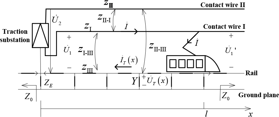
Figure 1: Circuit model of double-wire traction network.

Therefore, the impedance per unit length of the contact wire is

$$\begin{array}{c}{Z}_T^{\prime }=R_T^{\prime }+j\omega L_T^{\prime }=\frac{{\dot{U}}_1-{\dot{U}}_1^{\prime }}{\dot{I}l}\hfill \\ =\left(z_{\mathrm{I}}-\frac{z_{\mathrm{I}-\mathrm{III}}^2}{z_{\mathrm{III}}}\right)+\frac{{\left(z_{\mathrm{III}}-z_{\mathrm{I}-\mathrm{III}}\right)}^2}{2z_{\mathrm{III}}\sqrt{z_{\mathrm{III}}y}}\hfill \\ \cdot \left[\left(1-e^{-\gamma l}\right)-\frac{2Z_E+Z_0{e}^{-\gamma l}}{Z_0+2Z_E}\left(e^{-\gamma l}-1\right)\right]\cdot \frac{1}{l},\hfill \end{array}$$

(2)

where $\gamma$ is the propagation coefficient of the trail. $\gamma =\sqrt{z_{\mathrm{III}}y}$, and $Z_0=\sqrt{z_{\mathrm{III}}\mathrm{/}y}$. Traction network impedance includes linear components and nonlinear components. It can be seen that when $l$ is large, the nonlinear components can be ignored in a sinusoidal steady state circuit. However, when the current frequency is high, the nonlinear components cannot be ignored. $z_{\mathrm{I}}$, $z_{\mathrm{II}}$, $z_{\mathrm{III}}$, and $z_{\mathrm{I}-\mathrm{II}}$ can all be calculated according to the traction network parameters [25].

When the traction network is short-circuited, the contacts of the circuit breaker will be disconnected, and an arc will be generated. The arc will be extinguished when the current crosses zero. Circuit breaker arc is the main cause of high-frequency transient current and TEMF. The frequency of multiple reignitions caused by circuit breaker opening can reach 1 MHz [26]. The electromagnetic wave wavelength $\lambda$ is 300 m. Based on the lumped parameter model of the contact wire, we established a TCM for traction network short-circuit, as shown in Figure 2.

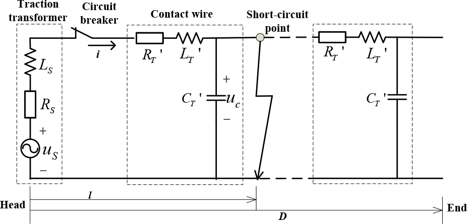
Figure 2: TCM for traction network short-circuit.

It includes traction transformers, circuit breakers, and contact wires. D is the length of a power supply arm, and the distance between the short-circuit point and the substation is l. $u_S$ is a 27.5 5-kV AC voltage source provided by the substation for the contact wire. $R_S$ and $L_S$ are the equivalent resistance and inductance of the transformer in the substation, respectively. They can be calculated by the electrical parameters of traction transformer.

$C_T^{\prime }$ is the capacitance per unit length of the contact line to the ground, and it is

$$C_T^{\prime }=\frac{2\pi {\epsilon }_0}{\ln \left(2h\mathrm{/}a\right)},$$

(3)

where $a$ and $h$ are the radius and height of the contact wire, and ${\epsilon }_0$ is the vacuum dielectric constant.

B. The transient current

Suppose that when $t=0$, the traction network is short-circuited, and when $t=t_1$, the contacts of the circuit breaker are disconnected. Before the traction network is short-circuited, the traction system works normally. The voltage on the contact wire is $u_S\left(t\right)=U_S\sin \left(\omega t+{\psi }_{0u}\right)$, and the frequency is 50 Hz. The impedance of the train body is $X$, while the equivalent resistance, equivalent inductance, and ground capacitance of the short-circuit point to the substation are $R_T$, $L_T$, and $C_T$, respectively. As a result, the current flowing across the contact wire is

$$i_{(t\le 0)}\left(t\right)=\frac{U_S\sin \left(\omega t+{\psi }_{0u}-{\phi }_0\right)}{\sqrt{{\left(R_S+R_T\right)}^2+{\left(\omega L_S+\omega L_T+\omega C_T-\frac{1}{X}\right)}^2}}.$$

(4)

The voltage on the $C_T$ is

$$u_{c(t\le 0)}\left(t\right)=\frac{U_S\left|\omega C_T-\frac{1}{X}\right|\cos \left(\omega t+{\psi }_{0u}-{\phi }_0\right)}{\sqrt{{\left(R_S+R_T\right)}^2+{\left(\omega L_S+\omega L_T+\omega C_T-\frac{1}{X}\right)}^2}},$$

(5)

where ${\psi }_{0u}$ is the initial phase of $u_s$, and ${\phi }_0$ is the phase difference between the voltage and current before the contact wire is short-circuited. So,

$$\tan {\phi }_0=\frac{\omega \left(L_S+L_T+CT\right)-\frac{1}{X}}{R_S+R_T}.$$

(6)

When $t=0$, the contact wire is short-circuited. According to Figure 2, the transient circuit can be expressed as

$\left(L_S+L_T\right)C_T{\displaystyle \frac{d^2{u}_c\left(t\right)}{dt}}+\left(R_S+R_T\right)$
$C_T{\displaystyle \frac{d{u}_c\left(t\right)}{dt}}+u_c\left(t\right)=u_S\left(t\right).$	(7)

According to the initial values provided by equation (4) and (5), the current $i\left(t\right)$ when $0<t\le t_1$ can be calculated, as

$i_{(0<t\le t_1)}\left(t\right)={\displaystyle \frac{U_S\cos \left(\omega t+{\psi }_{0u}-{\phi }_1\right)}{W_1}}$
$+A_1{P}_1{C}_T{e}^{P_{1}t}+A_2{P}_2{C}_T{e}^{P_{2}t},$	(8)

where ${\phi }_1$, $W_1$, $P_1$, $P_2$, $A_1$, and $A_2$ are,

$${\phi }_1=\arctan \frac{\omega \left(L_S+L_T\right)-\frac{1}{\omega C_T}}{R_S+R_T},$$

(9)

$$W_1=\sqrt{{\left(R_S+R_T\right)}^2+{\left(\omega \left(L_S+L_T\right)-\frac{1}{\omega C_T}\right)}^2},$$

(10)

$$P_1=-\frac{R_S+R_T}{2\left(L_S+L_T\right)}+\sqrt{{\left(\frac{R_S+R_T}{2\left(L_S+L_T\right)}\right)}^2-\frac{1}{\left(L_S+L_T\right)C_T}},$$

(11)

$$P_2=-\frac{R_S+R_T}{2\left(L_S+L_T\right)}-\sqrt{{\left(\frac{R_S+R_T}{2\left(L_S+L_T\right)}\right)}^2-\frac{1}{\left(L_S+L_T\right)C_T}},$$

(12)

$$A_1=\frac{1}{P_1-P_2}\left[W_2-P_2\left(W_3-\frac{U_S\sin \left({\psi }_{0u}-{\phi }_1\right)}{\omega C_T{W}_1}\right)\right],$$

(13)

$$A_2=\frac{1}{P_2-P_1}\left[W_2-P_1\left(W_3-\frac{U_S\sin \left({\psi }_{0u}-{\phi }_1\right)}{\omega C_T{W}_1}\right)\right].$$

(14)

In $A_1$ and $A_2$, $W_2$ and $W_3$ are, respectively,

$$\begin{array}{c}{W}_2=\frac{U_S\sin \left({\psi }_{0u}-{\phi }_0\right)}{C_T\sqrt{{\left(R_S+R_T\right)}^2+{\left(\omega L_S+\omega L_T+\omega C_T-\frac{1}{X}\right)}^2}}\hfill \\ -\frac{U_S\cos \left({\psi }_{0u}-{\phi }_1\right)}{C_T{W}_1},\hfill \end{array}$$

(15)

$$W_3=\frac{U_S\left|\omega C_T-\frac{1}{X}\right|\cos \left({\psi }_{0u}-{\phi }_0\right)}{\sqrt{{\left(R_S+R_T\right)}^2+{\left(\omega L_S+\omega L_T+\omega C_T-\frac{1}{X}\right)}^2}}.$$

(16)

When $t=t_1$, the contact of the circuit breaker is disconnected and an arc is generated. When the current crosses zero, the arc is extinguished, and the contact wire is truly disconnected. According to Figure 2, we can get,

$$L_S{C}_T\frac{d^2{u}_c\left(t\right)}{dt}+R_S{C}_T\frac{d{u}_c\left(t\right)}{dt}+u_c\left(t\right)=u_S\left(t\right).$$

(17)

Therefore, it can be deduced that the current when t $>$ 0 is

$$\begin{array}{c}{i}_{(t>t_1)}\left(t\right)=\frac{U_S\sin (\omega (t-t_1)+{\psi }_{0u}-{\phi }_1-{\phi }_2)}{\sqrt{R_S^2+{\left(\omega L_S-\frac{1}{\omega C_T}\right)}^2}}\hfill \\ +A_3{P}_3{C}_T{e}^{-P_3(t-t_1)}+A_4{P}_4{C}_T{e}^{-P_4(t-t_1)},\hfill \end{array}$$

(18)

where ${\phi }_2$, $P_3$, $P_4$, $A_3$, and $A_4$ are, respectively,

$${\phi }_2=\arctan \frac{\omega L_S-\frac{1}{\omega C_T}}{R_S},$$

(19)

$$P_3=-\frac{R_S}{2L_S}+\sqrt{{\left(\frac{R_S}{2L_S}\right)}^2-\frac{1}{L_S{C}_T}},$$

(20)

$$P_4=-\frac{R_S}{2L_S}-\sqrt{{\left(\frac{R_S}{2L_S}\right)}^2-\frac{1}{L_S{C}_T}},$$

(21)

$$A_3=\frac{1}{P_3-P_4}\left[\frac{i_{0<t\le t_1}\left(t_1\right)}{C_T}-P_4\left(W_5-W_4\right)\right],$$

(22)

$$A_4=\frac{1}{P_4-P_3}\left[\frac{i_{0<t\le t_1}\left(t_1\right)}{C_T}-P_3\left(W_5-W_4\right)\right].$$

(23)

In $A_3$ and $A_4$, $W_4$ and $W_5$ are, respectively,

$$W_4=\frac{U_S}{\sqrt{R_S^2+{\left(\omega L_S-\frac{1}{\omega C_T}\right)}^2}},$$

(24)

$$W_5=\frac{U_S\sin \left(\omega t_1+{\psi }_{0u}-{\phi }_1\right)}{\omega C_T{W}_1}+A_1{e}^{P_1{t}_1}+A_2{e}^{P_2{t}_1}.$$

(25)

After the arc is extinguished, the current quickly decays to zero. Through Fast Fourier Transform (FFT) transformation, the frequency spectrum of transient current can be obtained.

C. The transient electromagnetic field

The oscillating wave generated by the transient current becomes the disturbance source, radiating the TEMF energy to the surrounding space. When the distance between the short-circuit point and the substation is less than $\lambda \mathrm{/}4$, and the height between the circuit point and the ground is less than $\lambda \mathrm{/}4$, the current direction at all points on the line can be considered to be same. Therefore, we take the closed loop as a loop antenna and divide it into Q small circles, as shown in Figure 3. The radius of the small circle is $da$ and meets $da\ll \lambda$. The shielded cable head is P. The horizontal distance from the substation is $D_x$. $r_q$ is the distance from the q-th small circle to P. $D_y$ is the vertical distance between the shielded cable and the rail.

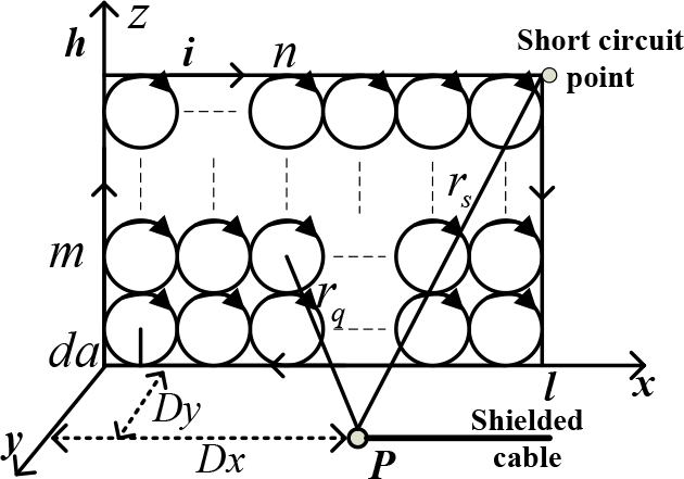
Figure 3: Segmentation calculation of the electromagnetic field in a loop circuit.

The electromagnetic field at P is the superposition of the electromagnetic fields generated by each small ring. $r_s$ is the distance from P to the short-circuit point, which can be expressed as

$$r_s=\sqrt{h^2+D_y^2+{\left|l-D_x\right|}^2}.$$

(26)

Let ${\varphi }_q$ be the angle between the $x$ x-axis and the projection of $r_q$ on the $xoy$ plane, and ${\theta }_q$ be the angle between $r_q$ and the $z$ z-axis. According to the electromagnetic field theory, when the shielded cable is in the near field of the radiation field, the electromagnetic field at P can be expressed as

$$E=\sum _{q=1}^{Q}d{E}_{{\varphi }_q}=\sum _{q=1}^Q-jk\eta \frac{Id{a}^2}{4r_q^2}\sin {\theta }_q{e}^{-jk{r}_q},$$

(27)

$H=$	${\displaystyle \sum _{q=1}^Q}\sqrt{d{H}_{r_q}^2+d{H}_{{\theta }_q}^2}$	(28)
	$=$	${\displaystyle \sum _{q=1}^Q}{\displaystyle \frac{Id{a}^2}{2r_q^3}}\sqrt{{\left(\cos {\theta }_q\right)}^2+{\displaystyle \frac{1}{4}}{\left(\sin {\theta }_q\right)}^2}\cdot e^{-jkr{}_q},$

where I and f are the effective value and frequency of the transient current, and $c$ is the speed of the wave in free space. $\eta \approx 377\mathrm{\Omega }$ for wave impedance in free space, $k=2\pi f\mathrm{/}c$ for propagation constant. Q small circles are represented in the form of a matrix. The distance between the small circle in m row and n column to P can be expressed as,

$$r_{mn}=\sqrt{{\left(\left(2m-1\right)da\right)}^2+D_y^2+{\left|D_x-\left(2n-1\right)da\right|}^2},$$

(29)

where $1\le m\le h\mathrm{/}2da$, $1\le n\le l\mathrm{/}2da$.

Let $D_{xx}=\left|D_x-\left(2n-1\right)da\right|$, $D_{xx}=\left|D_x-\left(2n-1\right)da\right|$; the TEMF at P can be expressed as

$$E=\sum _{m=1}^{h\mathrm{/}2da}\sum _{n=1}^{l\mathrm{/}2da}\frac{-j60{\pi }^{2}f\cdot Id{a}^2}{c{r}_{mn}^3}\sqrt{D_y^2+D_{xx}^2}\cdot e^{-jk{r}_{mn}},$$

(30)

$H={\displaystyle \sum _{m=1}^{h\mathrm{/}2da}}{\displaystyle \sum _{n=1}^{l\mathrm{/}2da}}{\displaystyle \frac{Id{a}^2}{2r_{mn}^4}}$
$\sqrt{{\left(2m-1\right)}^{2}d{a}^2+{\displaystyle \frac{1}{4}}{D}_y^2+{\displaystyle \frac{1}{4}}{D}_{xx}^2}\cdot e^{-jk{r}_{mn}}.$	(31)

It can be seen that the TEMF generated by the TNSF on the shielded cable is related to the height of the contact wire, the distance from the short-circuit point, the amplitude and frequency of the transient current, and the location of the shielded cable.

III. THE RESPONSE ON THE SHIELDED CABLE

If the cables of weak-current equipment are exposed, they are easily coupled by electromagnetic fields. Disturbance voltage and disturbance current are induced and enter the equipment along the inner conductor to cause EMI. We calculated the response of the TEMF on the shielded cable based on the transmission TL theory. A shielded cable includes a shielding layer and an inner conductor, which is defined as two independent transmission TLs. The electromagnetic field generates current and voltage on the shielding layer. The voltage and current on the shielding layer generate current and voltage on the inner conductor through transfer impedance and transfer admittance.

A. The voltage and current on the shielding layer

Let the incident angle, the azimuth angle, and the polarization angle of the electromagnetic field be $\phi$, $\psi$, and $\alpha$, respectively. The Agrawal model decomposes the incident field into the excitation field component that does not depend on the shielding structure and the scattered field component due to the induced charge and induced current on the shielding layer. Treating the shielding layer as an external transmission line (ETL), the equivalent circuit coupled to the shielding layer is shown in Figure 4. Cable length is L. $h_c$ is the height from the ground. $V_1$ and $V_2$ are the lumped voltage sources at the ETL’s two ends, and $V_S^{\prime }\left(x\right)$ is the excitation voltage source along the direction of the ETL. Load impedances at both ends of the ETL are $Z_{e1}$ and $Z_{e1}$, respectively. $Z_e^{\prime }$ and $Y_e^{\prime }$ are the ETL’s unit impedance and unit admittance, which can be calculated using the shielded cable’s parameters. The scattering field voltage is $V_{\mathrm{sc}}\left(x\right)$, the incident field is $E_{\mathrm{in}}$, and the ground reflection field is $E_{\mathrm{re}}$. $\widehat{k}$ represents the direction of the plane wave generated by the electromagnetic field.

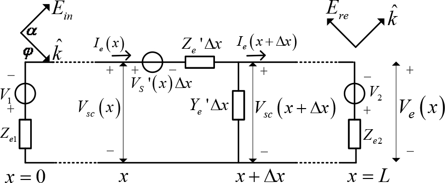
Figure 4: The equivalent circuit of the shielding layer.

Assume that the incident field spectrum is $E_0\left(\omega \right)$. According to the components of $E_{\mathrm{in}}$ and $E_{\mathrm{re}}$ along the ETL, $V_S^{\prime }\left(x\right)$, $V_1$, and $V_2$ can be deduced.

$$V_S^{\prime }\left(x\right)=jk2h_c{E}_0\left(\omega \right)\sin \phi \cdot \left(\begin{array}{c}\cos \alpha \sin \phi \cos \psi \hfill \\ +\sin \alpha \sin \psi \hfill \end{array}\right)e^{-j{k}_{x}x},$$

(32)

$$V_1\approx -2h_c{E}_0\left(\omega \right)\cos \alpha \cos \phi ,$$

(33)

$$V_2\approx V_1{e}^{-j\cos \phi \cos \psi kL},$$

(34)

where $k=2\pi \mathrm{/}\lambda$, $k=2\pi \mathrm{/}\lambda$ and $k_x=k\cos \phi \cos \psi$. From Figure 4, we can get

$$\frac{d}{dx}\left[\begin{array}{c}\hfill V_{\mathrm{sc}}\left(x\right)\hfill \\ \hfill I_e\left(x\right)\hfill \end{array}\right]+\left[\begin{array}{cc}\hfill 0\hfill & \hfill Z_e^{\prime }\hfill \\ \hfill Y_e^{\prime }\hfill & \hfill 0\hfill \end{array}\right]\left[\begin{array}{c}\hfill V_{\mathrm{sc}}\left(x\right)\hfill \\ \hfill I_e\left(x\right)\hfill \end{array}\right]=\left[\begin{array}{c}\hfill V_S^{\prime }\left(x\right)\hfill \\ \hfill 0\hfill \end{array}\right].$$

(35)

Referring to [27], the current $I_e\left(x\right)$ and scattered voltage $V_{\mathrm{sc}}\left(x\right)$ at the x of the TL can be expressed in the form of Green’s function. Therefore, $I_e\left(x\right)$ and $V_{\mathrm{sc}}\left(x\right)$ can be expressed as

$$I_e\left(x\right)=K_1{e}^{r_{e}x}+K_2{e}^{-r_{e}x}+K_3{e}^{-j\cos \phi \cos \psi kx},$$

(36)

$$V_{\mathrm{sc}}\left(x\right)=-\frac{1}{Y_e^{\prime }}\left[\begin{array}{c}{K}_1{r}_e{e}^{r_{e}x}-K_2{r}_e{e}^{-r_{e}x}\hfill \\ -jk\cos \phi \cos \varphi K_3{e}^{-j\cos \phi \cos \psi kx}\hfill \end{array}\right],$$

(37)

where $r_e=\sqrt{Z_e^{\prime }{Y}_e^{\prime }}$ is the propagation constant of the ETL. $K_1$, $K_2$, and $K_3$ are

$K_1={\displaystyle \frac{1}{2Z_{e0}\left[1-{\rho }_{e1}{\rho }_{e2}{e}^{-2r_{e}L}\right]}}$

$\left\{\begin{array}{c}{V}_x^{\prime }\left[\begin{array}{c}-e^{-r_e^{+}L}\left({\displaystyle \frac{1}{r_e^{+}}}+{\displaystyle \frac{{\rho }_{e1}}{r_e^{-}}}\right)\hfill \\ +{\rho }_{e2}{e}^{-2r_{e}L}\left({\displaystyle \frac{1}{r_e^{-}}}+{\displaystyle \frac{{\rho }_{e1}}{r_e^{+}}}\right)\hfill \end{array}\right]\hfill \\ +V_1\left[\begin{array}{c}\left(1-{\rho }_{e1}\right){\rho }_{e2}{e}^{-2r_{e}L}\hfill \\ +\left(1-{\rho }_{e2}\right)e^{-r_e^{+}L}\hfill \end{array}\right]\hfill \end{array}\right\},$

(38)

$K_2={\displaystyle \frac{1}{2Z_{e0}\left[1-{\rho }_{e1}{\rho }_{e2}{e}^{-2r_{e}L}\right]}}$

$\left\{\begin{array}{c}{V}_x^{\prime }\left[\begin{array}{c}{\rho }_{e1}{e}^{-r_e^{+}L}\left({\displaystyle \frac{1}{r_e^{+}}}+{\displaystyle \frac{{\rho }_{e1}}{r_e^{-}}}\right)\hfill \\ -\left({\displaystyle \frac{1}{r_e^{-}}}+{\displaystyle \frac{{\rho }_{e1}}{r_e^{+}}}\right)\hfill \end{array}\right]\hfill \\ -V_1\left[\begin{array}{c}\left(1-{\rho }_{e1}\right)\hfill \\ +\left(1-{\rho }_{e2}\right){\rho }_{e1}{e}^{-r_{e}L}\hfill \end{array}\right]\hfill \end{array}\right\},$

(39)

$$K_3=\frac{V_x^{\prime }}{2Z_{e0}}\left(\frac{1}{r_e^{-}}+\frac{1}{r_e^{+}}\right).$$

(40)

$V_x^{\prime }$ is

$$V_x^{\prime }=j2k{h}_c{E}_0\left(\omega \right)\sin \phi \left(\begin{array}{c}\cos \alpha \sin \phi \cos \psi \hfill \\ +\sin \alpha \sin \psi \hfill \end{array}\right).$$

(41)

$Z_{e0}=\sqrt{Z_e^{\prime }\mathrm{/}{Y}_e^{\prime }}$ is the characteristic impedance of the ETL. ${\rho }_{e1}$ and ${\rho }_{e2}$ are the reflection coefficients at the two ends of the ETL, and they are

$${\rho }_{e1}=\frac{Z_{e1}-Z_{e0}}{Z_{e1}+Z_{e0}},$$

(42)

$${\rho }_{e2}=\frac{Z_{e2}-Z_{e0}}{Z_{e2}+Z_{e0}}.$$

(43)

The propagation constants $r_e^{+}$ and $r_e^{-}$ are,

$$r_e^{+}=r_e+jk\cos \phi \cos \psi ,$$

(44)

$$r_e^{-}=r_e-jk\cos \phi \cos \psi .$$

(45)

The total voltage at the x of the TL is

$V_e\left(x\right)=V_{\mathrm{sc}}\left(x\right)-{\displaystyle {\int }_0^{h_c}}{E}_{\mathrm{in}}\mathit{d}z$
$=V_{\mathrm{sc}}\left(x\right)-h_c{E}_0\left(\omega \right)\cos \alpha \cos \phi .$	(46)

B. The voltage and current on the inner conductor

The current on the shielding layer penetrates into the shielded cable and generates an excitation source on the inner conductor. Taking the inner conductor as the Inner Transmission Line (ITL), its equivalent circuit model is shown in Figure 5.

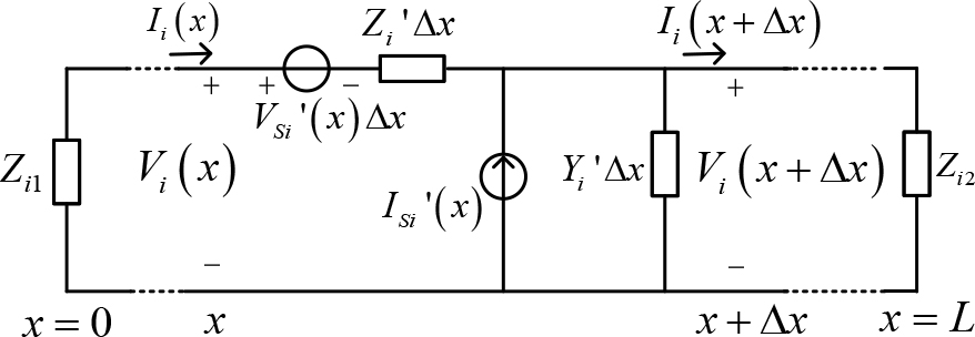
Figure 5: The equivalent circuit of the inner conductor.

Load impedances at both ends of the ITL are $Z_{i1}$ and $Z_{i2}$. $Z_i^{\prime }$ and $Y_i^{\prime }$ are the ITL’s unit impedance and unit admittance, which can be calculated using the shielded cable’s parameters. $V_{Si}^{\prime }\left(x\right)$ and $I_{Si}^{\prime }\left(x\right)$ are the excitation voltage source and current source on the ITL.

$$V_{Si}^{\prime }\left(x\right)=Z_t^{\prime }{I}_e,$$

(47)

$$I_{Si}^{\prime }\left(x\right)=-Y_t^{\prime }{V}_e,$$

(48)

where $Z_t^{\prime }$ and $Y_t^{\prime }$ are transfer impedance and transfer admittance, and their values refer to [28] and [29]. According to the Baum–Liu–Tesche (BLT) equation [30], the current and voltage at both ends of the ITL can be deduced as

$$\left[\begin{array}{c}\hfill I_i\left(0\right)\hfill \\ \hfill I_i\left(L\right)\hfill \end{array}\right]=\frac{1}{Z_{i0}}\left[\begin{array}{cc}\hfill 1-{\rho }_{i1}\hfill & \hfill 0\hfill \\ \hfill 0\hfill & \hfill 1-{\rho }_{i2}\hfill \end{array}\right]{\left[\begin{array}{cc}\hfill -{\rho }_{i1}\hfill & \hfill e^{r_{i}L}\hfill \\ \hfill e^{r_{i}L}\hfill & \hfill -{\rho }_{i2}\hfill \end{array}\right]}^{-1}\left[\begin{array}{c}\hfill S_{i1}\hfill \\ \hfill S_{i2}\hfill \end{array}\right],$$

(49)

$$\left[\begin{array}{c}\hfill V_i\left(0\right)\hfill \\ \hfill V_i\left(L\right)\hfill \end{array}\right]=\left[\begin{array}{cc}\hfill 1+{\rho }_{i1}\hfill & \hfill 0\hfill \\ \hfill 0\hfill & \hfill 1+{\rho }_{i2}\hfill \end{array}\right]{\left[\begin{array}{cc}\hfill -{\rho }_{i1}\hfill & \hfill e^{r_{i}L}\hfill \\ \hfill e^{r_{i}L}\hfill & \hfill -{\rho }_{i2}\hfill \end{array}\right]}^{-1}\left[\begin{array}{c}\hfill S_{i1}\hfill \\ \hfill S_{i2}\hfill \end{array}\right],$$

(50)

where $Z_{i0}$ is the characteristic impedance of the ITL. ${\rho }_{i1}$ and ${\rho }_{i2}$ are the reflection coefficients at the two ends of the ITL. $r_i=\sqrt{Z_i^{\prime }{Y}_i^{\prime }}$ is the propagation constant of the ITL. $S_{i1}$ and $S_{i2}$ can be obtained by integrating $V_{Si}^{\prime }\left(x\right)$ and $I_{Si}^{\prime }\left(x\right)$, which are

$S_{i1}={\displaystyle \frac{1}{2}}{K}_1\left(Z_t^{\prime }-Z_{ef}^{\prime }\right){\displaystyle \frac{e^{\left(r_i+r_e\right)L}-1}{r_i+r_e}}$
$+{\displaystyle \frac{1}{2}}{K}_2\left(Z_t^{\prime }+Z_{ef}^{\prime }\right){\displaystyle \frac{e^{\left(r_i-r_e\right)L}-1}{r_i-r_e}}$
$+{\displaystyle \frac{1}{2}}{K}_3\left(Z_t^{\prime }+Z_{ef}^{\prime }{\displaystyle \frac{j{k}_x}{r_e}}\right){\displaystyle \frac{e^{\left(r_i-j{k}_x\right)L}-1}{r_i-j{k}_x}},$	(51)

$S_{i2}={\displaystyle \frac{1}{2}}{e}^{r_{i}L}{K}_1\left(Z_t^{\prime }-Z_{ef}^{\prime }\right){\displaystyle \frac{e^{\left(r_e-r_i\right)L}-1}{r_e-r_i}}$
$-{\displaystyle \frac{1}{2}}{e}^{r_{i}L}{K}_2\left(Z_t^{\prime }-Z_{ef}^{\prime }\right){\displaystyle \frac{e^{-\left(r_i+r_e\right)L}-1}{r_i+r_e}}$
$-{\displaystyle \frac{1}{2}}{e}^{r_{i}L}{K}_3\left(Z_t^{\prime }-Z_{ef}^{\prime }{\displaystyle \frac{j{k}_x}{r_e}}\right){\displaystyle \frac{e^{-\left(r_i+j{k}_x\right)L}-1}{r_i+j{k}_x}},$	(52)

where $Z_{ef}^{\prime }=j{r}_e{r}_i{S}_s\mathrm{/}\omega$, $Z_{ef}^{\prime }=j{r}_e{r}_i{S}_s\mathrm{/}\omega$ and $k_x=k\cos \phi \cos \psi$. When ignoring the propagation loss of the ETL and the ITL, then $Z_{ef}^{\prime }=j{k}^2{S}_s\mathrm{/}\omega$. $S_s$ is the electrostatic shield leakage parameter of the shielded cable. Through the inverse FFT transform, the current response in the time domain can be obtained.

When the impedance of the shielded cable terminal load is $Z$, its power is

$$P_{\mathrm{dBW}}=10\lg \left(i_i{\left(t\right)}^2\cdot Z\right).$$

(53)

If $P_{\mathrm{dBW}}$ exceeds the rated power of the terminal load, the terminal load will be disturbed or even damaged.

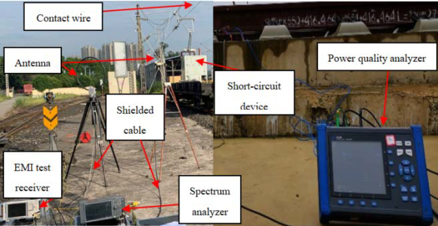
Figure 6: The experimental site.

IV. EXPERIMENT

The TNSF can be simulated by a short-circuit experiment, and the traction network short-circuitexperiment is realized by a short-circuit device and a high-voltage circuit breaker. The short-circuit device is composed of a pantograph, a high-voltage electrical cabinet, and a short-circuit grounding shoe. It is placed at the short-circuit point to realize the connection between the contact wire and the rail. The experimental site is shown in Figure 6. The power quality analyzer (E6100) is used to test the short-circuit current. The EMI test receiver is used to test the current generated by the low-frequency magnetic field, and the spectrum analyzer is used to test the voltage generated by the high-frequency electric field. The distance from the short-circuit point to the substation is 30 m. The length of the shielded cable is 5 m, the height of the head is 1 m, and the vertical distance from the rail is 2 m. The impedance of the spectrum analyzer is 50 $\mathrm{\Omega }$, and the rated power is 30 dBm. The traction network short-circuit experiment process is shown in Figure 7.

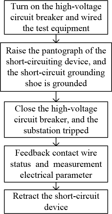
Figure 7: Traction network short-circuit experiment process.

Based on the actual traction network parameters, we calculate the transient current and the response of the shielded cable through the method proposed in Sections II and Section III. The calculated results are compared with the experimental results. The EMI on the terminal load is also analyzed.

A. Transient current

In the short-circuit experiment, the traction network’s power supply is a direct power supply with a return line. Contact wire (CW), messenger wire (MW), return wire (RW), and rail (R) make up the majority of the traction network. These conductors are distributed in parallel. Tables 1 and Table 2 show the major parameters of the traction transformer and traction network conductors in the experiment. Figure 8 shows the traction network’s spatial distribution.

Table 1: Major parameters of the traction transformer

Parameters	Value
Short-circuit losses	146.49 kW
Short-circuit voltage	16.48 %
Rated voltages	220/2 $\times$ 27.5 kV
Rated current	227.27/909.08 A

Table 2: Major parameters of traction networkconductors

Conductor	Type	DC resistance ($\mathrm{\Omega }$/km)	Calculate radius (cm)
CW1/ CW2	CTS-150	0.159	0.72
MW1/MW2	JTMH-120	0.242	0.70
RW1/RW2	LBGLJ-185/25	0.145	0.945
R1/ R2	P60	0.135	1.279

The parameters of the TCM in Figure 2 can be calculated using the distance between the traction network conductors and the parameters in Tables 1 and Table 2, as shown in Table 3.

When a short-circuit fault occurs, let the initial phase angle of $u_s$ be 0${}^{\circ }$ and the duration of the short-circuit process be 0.15 s. Figure 9 shows the computed and measured values of the short-circuit current in the time domain.

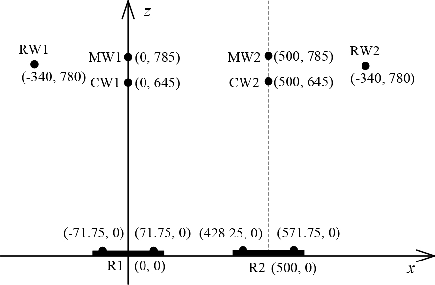
Figure 8: Spatial distribution of traction network conductors (unit: cm).

Table 3: Equivalent component parameters of TCM

Circuit component	Value
R${}_S$	0.18 $\mathrm{\Omega }$
L${}_S$	32 mH
$R_T^{\prime }$	0.335 $\mathrm{\Omega }$/ km
$L_T^{\prime }$	0.2944 $\mathrm{\Omega }$/ km
$C_T^{\prime }$	0.0074 $\mu$F / km

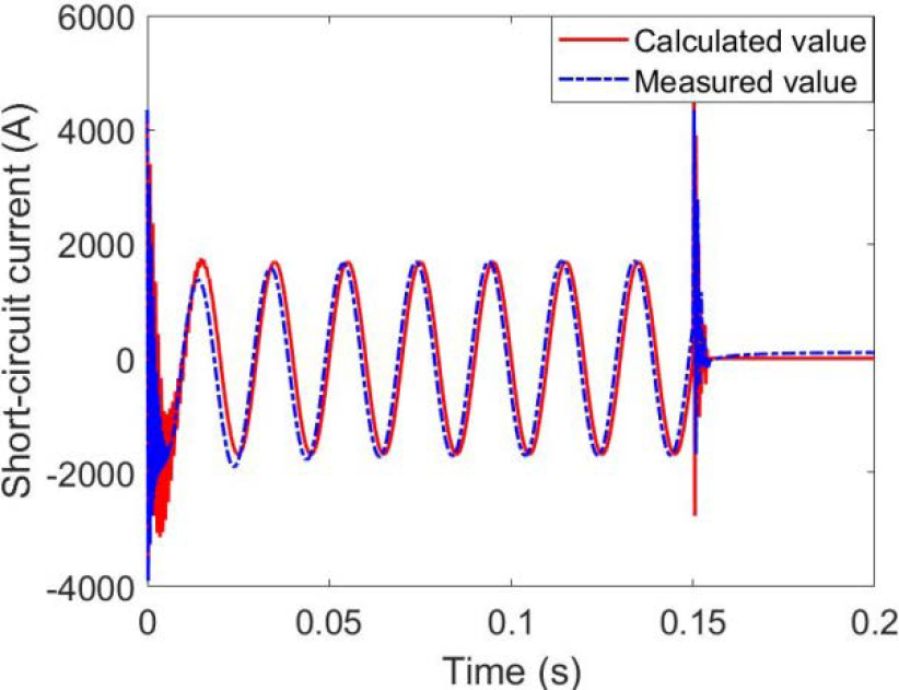
Figure 9: Short-circuit current.

It can be seen that when a TNSF occurs, there is a small error between the calculated value and the measured value of the short-circuit current phase and amplitude. Since the actual circuit breaker has an arc extinguishing device, the calculated value is greater than the measured value. However, the waveform of the short-circuit current calculated value is in good agreement with the measured waveform. The maximum value of the short-circuit current is about 1644 A, the maximum value of the transient current is about 4351 A, and the duration of the transient process is about 0.015 s. The transient process of short-circuiting and circuit breaker opening produces a high-frequency current, and the frequency component of the measured data is more complicated due to the contingency of the arc in the actual test.

B. The terminal current of the shielded cable

When calculating the current response of the shielded cable, the height of the contact wire and the distance from the shielded cable head to the short-circuit point are the same as in the actual test experiment. The radius of the small circle is 0.005 m. The type of the shielded cable in the experiment is RG-214(I), and its major parameters are shown in Table 4. Both ends of the shielding layer are grounded through the antenna and the instrument casing. The impedance of the inner conductor matches the characteristic impedance of the shielded cable, which is 50 $\mathrm{\Omega }$.

Table 4: Major parameters of shielded cable

Parameter	Value
The radius of the shield	0.37 cm
The thickness of the shield	0.127 mm
DC resistance	4.0 m$\mathrm{\Omega }$ / m
Hole inductance	0.25 nH / m
leakage parameters	16 m /$\mu \mathrm{F}$

When the incident angle, azimuth angle, and polarization angle of the electromagnetic field are, respectively, 30${}^{\circ }$, 0${}^{\circ }$, and 0${}^{\circ }$, and $D_x$ is 10 m, the calculated and measured values of the shielded cable terminal current at some frequency points are shown in Table 5. It can be seen that the calculated values are in good agreement with the measured values, which verifies the method in this article. The higher the frequency, the smaller the current response. The value is larger when the current is below 1 MHz.

Table 5: The calculated and measured value of the current response

Frequency (MHz)	Calculated value (dB$\mu$A)	Measured value (dB$\mu$A)
0.01	49.83	50.09
0.1	48.65	46.67
0.5	47.75	46.65
1	34.55	33.62
5	21.05	20.83
10	17.3	14.82
20	14.15	11.19
30	$-$18.66	$-$18.88
40	$-$21.69	$-$20.28
50	$-$26.60	$-$25.68

C. Analysis of EMI on terminal load

The current response of the shielded cable generates power on the shielded cable terminal load. If the power exceeds its rated power, the terminal load will be disturbed or even destroyed. We calculate the power of the shielded cable terminal load under different conditions and analyze the EMI of the transient magnetic field generated by TNSF on the shielded cable terminal load.

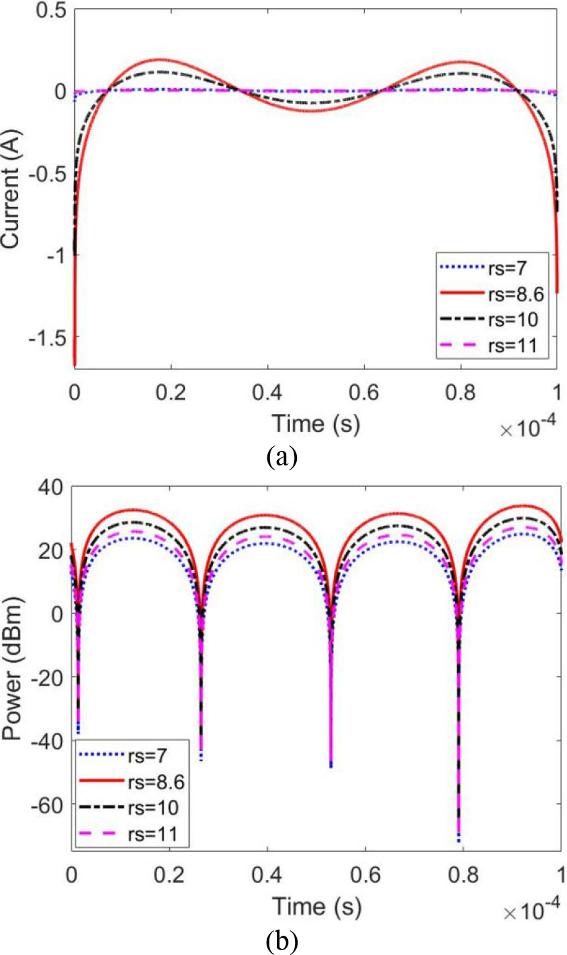
Figure 10: (a) Terminal current of shielded cable under different $r_s.$ (b) Spectrum analyzer power underdifferent $r_s.$

Assume that the incident angle, azimuth angle, and polarization angle of the electromagnetic field are 30${}^{\circ }$, 0${}^{\circ }$, and 0${}^{\circ }$, respectively. When the distance between the shielded cable head and the short-circuit point is 7 m, 8.6 m, 10 m, and 11 m, respectively, the terminal current response of the shielded cable is shown in Figure 10 (a). The power generated by the terminal current on the spectrum analyzer is shown in Figure 10 (b). The fluctuations and discontinuities of the current waveform and power waveform in the figure are caused by the reflection of the current in the cable. It can be seen that when $r_s$ is 8.6 m, the terminal current reaches its maximum value of 0.1879 A, and then the terminal current decreases as $r_s$ increases. The maximum power can reach 32.33 dBm, which exceeds the rated power of the spectrum analyzer. According to equation (26), the horizontal distance between the shielded cable head and the short-circuit point must be more than 6 m to avoid damaging the spectrum analyzer.

Figure 11: Spectrum analyzer power under different incident angles.

If the distance between the shielded cable head and the short-circuit point is 8.6 m, the azimuth angle and the polarization angle are both 0${}^{\circ }$. When the incident angles are 0${}^{\circ }$, 45${}^{\circ }$, 60${}^{\circ }$, and 90${}^{\circ }$, the power of the spectrum analyzer is shown in Figure 11. It can be seen that the larger the incident angle, the smaller the terminal load power. When the incident angle is 45${}^{\circ }$, the power is 30.58 dBm, which exceeds the rated power of the spectrum analyzer. In order to avoid damage to the spectrometer, the incident angle should be greater than 45${}^{\circ }$.

If the distance between the shielded cable head and the short-circuit point is 8.6 m, the incident angle is 30${}^{\circ }$, and the polarization angle is 0${}^{\circ }$. When the azimuth angles are 0${}^{\circ }$, 45${}^{\circ }$, 60${}^{\circ }$, and 90${}^{\circ }$, the power of the spectrum analyzer is shown in Figure 12. The maximum power can reach 33.55 dBm, which also exceeds the rated power of the spectrum analyzer. The azimuth angle has less influence on the terminal load power. But when amplifying a part of the power waveform, it can be seen that the larger the azimuth angle, the smaller the power generated on the terminal load.

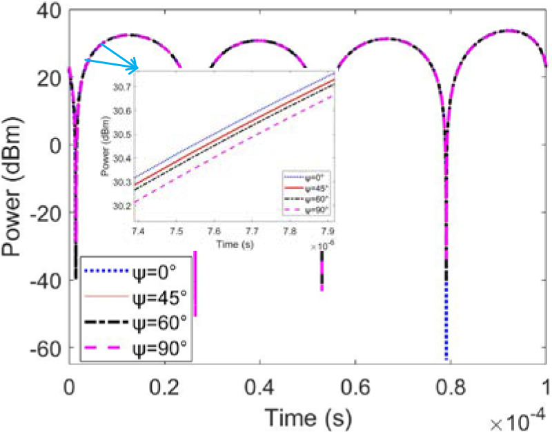
Figure 12: Spectrum analyzer power under different azimuth angles.

Figure 13: Spectrum analyzer power under different polarization angles.

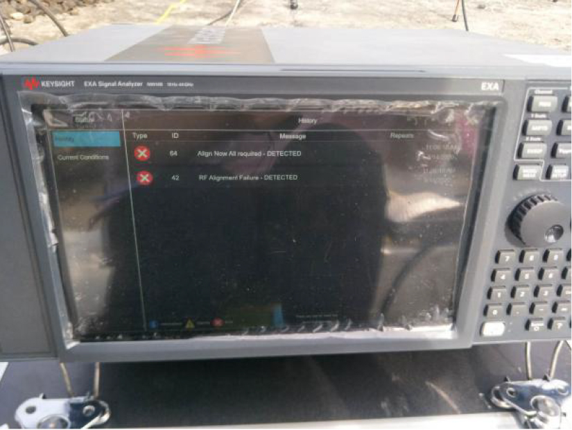
Figure 14: Damaged spectrum analyzer.

If the distance between the shielded cable head and the short-circuit point is 8.6 m, the incident angle is 30${}^{\circ }$, and the azimuth angle is 0${}^{\circ }$. When the polarization angles are 0${}^{\circ }$ and 90${}^{\circ }$, the spectrum analyzer power generated by the terminal current is shown in Figure 13. It can be seen that, compared with the vertical polarization mode, the terminal load power in the horizontal polarization mode is smaller.

Let the polarization angle be 0${}^{\circ }$, the azimuth angle be less than 90${}^{\circ }$, and the incident angle be less than 45${}^{\circ }$. We changed the relative position of the shielded cable and the short-circuit point to conduct many experiments. When the horizontal distance between the shielded cable head and the short-circuit point is about 5.3 m, the power generated by the terminal current of the shielded cable on the spectrum analyzer exceeds its rated power, which damages the RF input port of the spectrum analyzer. As shown in Figure 14.

V. CONCLUSION

1) This paper proposed a TCM for the short-circuit traction network to calculate the transient current. The model is validated by comparing the calculated and measured short-circuit current. The maximum value of transient current is about 4351 A, while the short-circuit current peaks at roughly 1644 A, and the transient process lasts about 0.015 s.

2) The TEMF was formed by the TCP caused by the TNSF. The current response of the TEMF on the shielded cable is calculated using transmission lineTL theory and verified by experiments. The horizontal distance between the shielded cable head and the short-circuit point should be greater than 6 m to avoid damaging the terminal load.

3) The change in the relative location of the shielded cable and the contact wire will cause the TEMF angle to shift. The larger the incident angle and the azimuth angle, the smaller the terminal load power will be. The azimuth angle has little effect on the terminal load power. When the polarization angle is 0${}^{\circ }$, greater power is generated on the terminal load. Therefore, to avoid damage to the terminal load, the incident angle should be greater than 45${}^{\circ }$.

ACKNOWLEDGMENT

The work was supported by National Key R&D Program of China under Grant No. 2018YFC0809500.

REFERENCES

[1] H. Xie, J. Wang, R. Fan, and Y. Liu, “A Hybrid FDTD-SPICE Method for Transmission Lines Excited by a Nonuniform Incident Wave,” IEEE Transactions on Electromagnetic Compatibility, vol. 51, no. 3, pp. 811-817, Aug. 2009.

[2] B. X. Zhang, P. Xiao, D. Ren, and P. A. Du, “An Analytical Method for Calculating Radiated Emission of Discontinuous Penetrating Cable,” The Applied Computational Electromagnetics Society (ACES) Journal, vol. 34, no. 01, pp. 25-32, 2021.

[3] G. Zhang, J. Bai, L. Wang, and X. Peng, “Stochastic Analysis of Multi-conductor Cables with Uncertain Boundary Conditions,” The Applied Computational Electromagnetics Society (ACES) Journal, vol. 33, no. 08, pp. 847-853, 2021.

[4] H. Xie, J. Wang, R. Fan, and Y. Liu, “SPICE Models to Analyze Radiated and Conducted Susceptibilities of Shielded Coaxial Cables,” IEEE Transactions on Electromagnetic Compatibility, vol. 52, no. 1, pp. 215-222, Feb. 2010.

[5] H. Xie, J. Wang, R. Fan, and Y. Liu, “SPICE Models for Prediction of Disturbances Induced by Nonuniform Fields on Shielded Cables,” IEEE Transactions on Electromagnetic Compatibility, vol. 53, no. 1, pp. 185-192, Feb. 2011.

[6] S. R. Huang, Y. L. Kuo, B. N. Chen, K. C. Lu, and M. C. Huang, “A short-circuit current study for the power supply system of Taiwan railway,” IEEE Transactions on Power Delivery, vol. 16, no. 4, pp. 492-497, Oct. 2001.

[7] X. Tian, X. Li, and Y. Li, “Current Waveform Feature and Fault Identification for Overhead Contact Line in Electrified Railway,” 2010 International Conference on Electrical and Control Engineering, 2010, pp. 3516-3519.

[8] C. Tejada, P. Gomez, and J. C. Escamilla, “Computation of Radio Interference Levels in High Voltage Transmission Lines with Corona,” IEEE Latin America Transactions, vol. 7, no. 1, pp. 54-61, March 2009.

[9] T. Lu, Y. Zou, H. Rao, and Q. Wang, “Analysis of electromagnetic radiation from HVAC test transmission line due to corona discharge,” Digests of the 2010 14th Biennial IEEE Conference on Electromagnetic Field Computation, 2010, pp. 1-1.

[10] V. $\check{\mathrm{S}}$midl, $\check{\mathrm{S}}$. Janou$\check{\mathrm{s}}$, and Z. Peroutka, “Improved Stability of DC Catenary Fed Traction Drives Using Two-Stage Predictive Control,” IEEE Transactions on Industrial Electronics, vol. 62, no. 5, pp. 3192-3201, May 2015.

[11] Y. X. Sun, Q. Li, W. H. Yu, Q. H. Jiang, and Q. K. Zhuo, “Study on Crosstalk Between Space Transient Interference Microstrip Lines Using Finite Difference Time Domain Method.” The Applied Computational Electromagnetics Society (ACES) Journal, vol. 30, no. 08, pp. 891-897, 2021.

[12] Z. Liu, G. Zhang and Y. Liao, “Stability Research of High-Speed Railway EMUs and Traction Network Cascade System Considering Impedance Matching,” IEEE Transactions on Industry Applications, vol. 52, no. 5, pp. 4315-4326, Sept.-Oct. 2016.

[13] R. Ianconescu and V. Vulfin, “Simulation and theory of TEM transmission lines radiation losses,” 2016 IEEE International Conference on the Science of Electrical Engineering (ICSEE), 2016, pp. 1-4.

[14] P. Taheri, B. Kordi and A. M. Gole, “Electric field radiation from an overhead transmission line located above a lossy ground,” 2008 43rd International Universities Power Engineering Conference, 2008, pp. 1-5.

[15] Q. Jin, W. Sheng, C. Gao, and Y. Han, “Internal and External Transmission Line Transfer Matrix and Near-Field Radiation of Braided Coaxial Cables,” IEEE Transactions on Electromagnetic Compatibility, vol. 63, no. 1, pp. 206-214,Feb. 2021.

[16] H. Lu, F. Zhu, Q. Liu, X. Li, Y. Tang, and R. Qiu, “Suppression of Cable Overvoltage in a High-Speed Electric Multiple Units System,” IEEE Transactions on Electromagnetic Compatibility, vol. 61, no. 2, pp. 361-371, April 2019.

[17] C. D. Taylor, R. S. Satterwhite, and C. W. Harrison, “The response of a treminated two-wire transmission line excited by a nonuniform electromagnetic field,” IEEE Trans. Antennas Propag., vol. AP-13, no. 6, pp. 987-989, Nov. 1965.

[18] A. K. Agrawal, H. J. Price, and S. H. Gurbaxani, “Transient response of multiconductor transmission lines excited by a nonuniform electromagnetic field,” IEEE Trans. Electromagn. Compat., vol. 22, no. 2, pp. 119-129, May 1980.

[19] F. Rachidi, “Formulation of the field-to-transmission line coupling equations in terms of magnetic excitation fields,” IEEE Trans. Electromagn. Compat., vol. 35, no. 3, pp. 404-407, Aug. 1993.

[20] F. Rachidi, “A Review of Field-to-Transmission Line Coupling Models With Special Emphasis to Lightning-Induced Voltages on Overhead Lines,” IEEE Transactions on Electromagnetic Compatibility, vol. 54, no. 4, pp. 898-911, Aug. 2012.

[21] X. Li, F. Zhu, H. Lu, R. Qiu, and Y. Tang, “Longitudinal Propagation Characteristic of Pantograph Arcing Electromagnetic Emission With High-Speed Train Passing the Articulated Neutral Section,” IEEE Transactions on Electromagnetic Compatibility, vol. 61, no. 2, pp. 319-326, April 2019.

[22] M. $\check{\mathrm{S}}$tumpf, “Pulsed EM Plane-Wave Coupling to a Transmission Line Over Orthogonal Ground Planes: An Analytical Model Based on EM Reciprocity,” IEEE Transactions on Electromagnetic Compatibility, vol. 63, no. 1, pp. 324-327, Feb. 2021.

[23] B. van Leersum, J. van der Ven, H. Bergsma, F. Buesink, and F. Leferink, “Protection Against Common Mode Currents on Cables Exposed to HIRF or NEMP,” IEEE Transactions on Electromagnetic Compatibility, vol. 58, no. 4, pp. 1297-1305, Aug. 2016.

[24] J. R. Carson, “Wave propagation in overhead wires with ground return,” The Bell System Technical Journal, vol. 5, no. 4, pp. 539-554, Oct. 1926.

[25] G. S. Lin and Q. Z. Li, “Impedance Calculations for AT Power Traction Networks with Parallel Connections,” 2010 Asia-Pacific Power and Energy Engineering Conference, 2010, pp. 1-5.

[26] Y. G. Li, ATP-EMTP and its application in power systems. Beijing, China:China Electric Power Press, 2016.

[27] F. M. Tesche, Plane Wave Coupling to Cables. New York, USA: Academic Press, 1995.

[28] E. F. Vance, Coupling to Shielded Cables. R. E. Krieger, Melbourne, FI, 1987.

[29] B. J. Zhang, G. Wang, L. Duffy, A. Liu, and T. Shao, “Comparison of Calculation Methods of Braided Shield Cable Transfer Impedance Using FSV Method, ” The Applied Computational Electromagnetics Society (ACES) Journal, vol. 30, no. 02, pp. 140-147, 2021.

[30] F. M. Tesche, and T. K. Liu, “Application of Multiconductor Transmission Line Network Analysis to Interaction Problems, ” Electromagnetics, vol. 6, no. 1, pp. 1-20, 1986.

BIOGRAPHIES

Yingchun Xiao was born in Gansu Province, China, in 1990. She received the B.S. degree in electronic information science and technology from the Lanzhou University of Technology, Lanzhou, China, in 2012, and is currently working toward the Ph.D. degree in electrical engineering at with Southwest Jiaotong University, Chengdu, China. At the same time, she is a lecturer Lecturer at with Lanzhou City College.

Her research interests include electromagnetic environment test and evaluation, electromagnetic compatibility analysis and design, and identification and location of electromagnetic interference sources.

Feng Zhu received the Ph.D. degree in railway traction electrification and automation from the Southwest Jiaotong University, Sichuan, China, in 1997.

He is currently a Full Professor with the School of Electrical Engineering, Southwest JiaotongUniversity.

His current research interests include locomotive over-voltage and grounding technology, electromagnetic theory and numerical analysis of electromagnetic field, and electromagnetic compatibility analysis anddesign.

Shengxian Zhuang received the M.S. and Ph.D. degrees from Southwest Jiaotong University and the University of Electronic Science and Technology of China in 1991 and 1999, respectively.

He is currently working with the School of Electrical Engineering at, Southwest Jiaotong University as a Professor. He got his M.S and Ph.D degrees, respectively, at Southwest Jiaotong University and the University of Electronic Science and Technology of China in 1991 and 1999. From 1999 to 2003, he did postdoctoral research at Zhejiang University and Linkoing University of Sweden. He was a visiting Professor at with Paderborn University in Germany in 2005 and at with the University of Leeds, U.K., in 2017.

His research interests include power conversion for sustainable energies, motor control and drive systems, power electronics and systems integration, and modeling, diagnosis, and suppression of electromagnetic interference of power electronic converters.

Yang Yang was born in Shanxi, China on April 19, 1989. She received her the bachelor’s degree in measurement and control technology and instrumentation from the Shaanxi University of Science and Technology in 2011 and her the master’s degree in control theory and control engineering from Northwestern Polytechnical University in 2014. She is currently working toward a the Ph.D. degree in electrical engineering at with Southwest Jiaotong University, Chengdu, China.

Her research interests include electromagnetic environment testing and evaluation, electromagnetic compatibility analysis and design, and electromagnetic compatibility problems in the field of railway power supply and rail transit.

ACES JOURNAL, Vol. 37, No. 4, 485–496.
doi: 10.13052/2022.ACES.J.370414
© 2021 River Publishers

Abstract

I. INTRODUCTION

II. THE TRANSIENT PROCESS OF THE SHORT-CIRCUIT TRACTION NETWORK

A. TCM for short-circuit traction network

B. The transient current

C. The transient electromagnetic field

III. THE RESPONSE ON THE SHIELDED CABLE

A. The voltage and current on the shielding layer

B. The voltage and current on the inner conductor

IV. EXPERIMENT

A. Transient current

B. The terminal current of the shielded cable

C. Analysis of EMI on terminal load

V. CONCLUSION

ACKNOWLEDGMENT

REFERENCES

BIOGRAPHIES