Low-Frequency Transmitted Fields of a Source Inside a Magnetic Shell with Large Conductivity

Shifeng Huang, Gaobiao Xiao, and Junfa Mao

¹Key Laboratory of Ministry of Education of Design and Electromagnetic Compatibility of High Speed Electronic Systems

²Shanghai Jiao Tong University, Shanghai 200240, China
huangshifeng@sjtu.edu.cn; gaobiaoxiao@sjtu.edu.cn; jfmao@sjtu.edu.cn

Submitted On: January 14, 2022; Accepted On: March 23, 2022

Abstract

The method to evaluate the transmitted fields of a source inside a simply connected magnetic shell with large but finite conductivity at low frequencies is proposed in this paper. When modeling the magnetic shell with large conductivity, it is regarded as a penetrable object. Electric field integral equation (EFIE) is selected for the exterior region problem and magnetic field integral equation (MFIE) is chosen for the interior region problem. Each operator is decomposed with loop-star functions to overcome the problem of low-frequency breakdown. Numerical results verify the accuracy of the proposed method.

Keywords: Large conductivity, loop-star, low frequency, magnetic material, transmitted fields.

I. INTRODUCTION

The analysis of electromagnetic compatibility (EMC) is frequently carried out to keep a system or components of a system working properly [1, 2]. For example, components of a microelectronic system should work normally and not interfere with others at the same time. The protection of an electronic system with high sensitivity from the electromagnetic (EM) emission from a high power electrical equipment is usually needed on a platform like ships and airplanes. One common strategy to suppress EM interference (EMI) is to enclose the electronic or electrical equipment with a shield with large conductivity if possible. Hence, it is necessary to calculate the fields transmitted from a shielding shell. In some scenarios, the amplitude of EM fields leaked from a target is expected to be as small as possible so that it cannot be detected. This is of great importance for some underwater targets, such as submarines and unmanned underwater vehicles. Because those underwater targets are immersed in sea water, low-frequency EM waves can propagate to a large distance. The body of underwater targets may be filled with magnetic materials. At low frequencies, the shell cannot be modeled as perfect electrical conductor (PEC) because the skin depth is comparable to its thickness. Hence, it is necessary to model the fields transmitted from a magnetic shell with large but finite conductivity accurately at low frequencies.

The method based on quasi-static approximation is first developed by neglecting the displacement currents [3, 4]. However, this approximate method can only work well at low frequencies and may give wrong results at relatively higher frequencies, and the frequency when quasi-static method fails is difficult to predict.

Rigorous methods are proposed to model conductor with large but finite conductivity, like finite element method (FEM), volume integral equation (VIE) method, and surface integral equation (SIE) method. SIE method is preferred to model conductors with the advantage of only discretizing the surface of conductors. In SIE method, the conductor is modeled as a penetrable object. Appropriate equations from the interior and exterior problems are selected to describe the behavior of the fields in the interior of the conductor and the coupling between other objects, respectively [5–8]. Examples are the method using the generalized impedance boundary condition (GIBC) [7] and the differential surface admittance (DSA) [8].

The low-frequency breakdown (LFB) problem of electric field integral operator (EFIO) in the SIE method mentioned above has to be overcome. Some remedies have been proposed. The primal and dual projectors of solenoidal and non-solenoidal component are used to perform quasi-Helmholtz decomposition of operators in Poggio-Miller-Chang-Harrington-Wu-Tsai (PMCHWT) equation [9]. Two low-frequency stable equations with different augment techniques are proposed in [10] and [11]. To reduce the number of equivalent surface sources on the interface and improve the efficiency of solvers, single-source formulations are proposed with augment techniques for lossy conductors to cover the low-frequency band analysis [12, 13]. Well-conditioned formulation based on potential, instead of electric and magnetic fields, is also reported to model good conductors [14].

In this work, the electric field integral equation (EFIE) in the exterior problem and the magnetic field integral equation (MFIE) in the interior problem of a shell are selected to model the shell with large conductivity and relative permeability, similar to [7]. The background media may also have large constitutive parameters, like sea water with large relative permittivity. Hence, PMCHWT equation are not chosen because it may fail to model objects with high contrast material parameters. The shell is thin with a thickness of several centimeters. The approximation in [7] due to small skin depth does not hold in this work because the skin depth may be comparable to the thickness. Furthermore, the LFB problem in [7] is not fully considered. Here, loop-star decomposition is performed on each operator in the equation for a simply connected shell. The low-frequency scaling of the decomposed coefficient matrix is analyzed and two sets of new rescaling coefficients are applied to improve the conditioning of the formular at low frequencies.

II. FORMULATION FOR THE SHELL

A. Equation formular at high frequency

A source in a magnetic shell with large but finite conductivity is shown in Figure 1. The source ${\mathbf{J}}^{\mathrm{in}}$ is in region $V_1$ with parameters $({\mu }_{r1},{\epsilon }_{r1},{\sigma }_1)$ and bounded by surface $\partial V_1$. Region $V_2$ denotes the shell with parameters $({\mu }_{r2},{\epsilon }_{r2},{\sigma }_2)$. The shell is bounded by surfaces $\partial V_1$ and $\partial V_2$. The shell is immersed in a homogeneous background media $V_3$ with parameters $({\mu }_{r3},{\epsilon }_{r3},{\sigma }_3)$. $\widehat{\mathbf{n}}$ is the outward unit vector of the surface. In our application, region $V_1$ is air with ${\sigma }_1=0$, region $V_2$ has large conductivity ${\sigma }_2$ and relative permeability ${\mu }_{r2}$, and region $V_3$ is sea water with large relative permittivity ${\epsilon }_{r3}$ and ${\sigma }_3=4S\mathrm{/}m$.

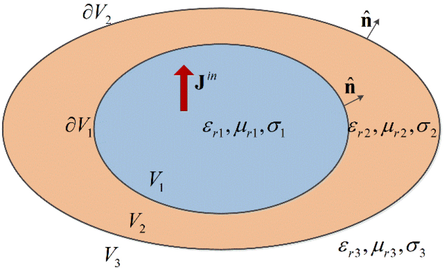
Figure 1: Configuration of a source in a shell immersed in a homogeneous background media.

Based on extinction theorem, the EFIE and MFIE describing the internal problem of region $V_1$ can bewritten as

$$\widehat{\mathbf{n}}\times \left[{ℒ}_{1E}\left\{{\mathbf{J}}_d^{1-}\right\}-{𝒦}_{1E}\left\{{\mathbf{M}}_d^{1-}\right\}+{\mathbf{E}}^{\mathrm{in}}\right]=0,\mathbf{r}\in \partial V_1,$$

(1)

and

$$\widehat{\mathbf{n}}\times \left[{𝒦}_{1H}\left\{{\mathbf{J}}_d^{1-}\right\}-{ℒ}_{1H}\left\{{\mathbf{M}}_d^{1-}\right\}+{\mathbf{H}}^{\mathrm{in}}\right]=0,\mathbf{r}\in \partial V_1,$$

(2)

where ${\mathbf{J}}_d^{1-}$ and ${\mathbf{M}}_d^{1-}$ are the unknown equivalent surface electric current and magnetic current density on $\partial V_1$. ${\mathbf{E}}^{\mathrm{in}}$ and ${\mathbf{H}}^{\mathrm{in}}$ are the fields radiated by the source ${\mathbf{J}}^{\mathrm{in}}$. The EFIE and MFIE describing the internal problem for region $V_2$ can be expressed as

$$\widehat{\mathbf{n}}\times \left[\begin{array}{c}{ℒ}_{2E}\left\{{\mathbf{J}}_d^{1+}\right\}-{𝒦}_{2E}\left\{{\mathbf{M}}_d^{1+}\right\}\hfill \\ +{ℒ}_{2E}\left\{{\mathbf{J}}_d^{2-}\right\}-{𝒦}_{2E}\left\{{\mathbf{M}}_d^{2-}\right\}\hfill \end{array}\right]=0,\mathbf{r}\in \partial V_1,$$

(3)

$$\widehat{\mathbf{n}}\times \left[\begin{array}{c}{ℒ}_{2E}\left\{{\mathbf{J}}_d^{1+}\right\}-{𝒦}_{2E}\left\{{\mathbf{M}}_d^{1+}\right\}\hfill \\ +{ℒ}_{2E}\left\{{\mathbf{J}}_d^{2-}\right\}-{𝒦}_{2E}\left\{{\mathbf{M}}_d^{2-}\right\}\hfill \end{array}\right]=0,\mathbf{r}\in \partial V_2,$$

(4)

and

$$\widehat{\mathbf{n}}\times \left[\begin{array}{c}{𝒦}_{2H}\left\{{\mathbf{J}}_d^{1+}\right\}-{ℒ}_{2H}\left\{{\mathbf{M}}_d^{1+}\right\}\hfill \\ +{𝒦}_{2H}\left\{{\mathbf{J}}_d^{2-}\right\}-{ℒ}_{2H}\left\{{\mathbf{M}}_d^{2-}\right\}\hfill \end{array}\right]=0,\mathbf{r}\in \partial V_1,$$

(5)

$$\widehat{\mathbf{n}}\times \left[\begin{array}{c}{𝒦}_{2H}\left\{{\mathbf{J}}_d^{1+}\right\}-{ℒ}_{2H}\left\{{\mathbf{M}}_d^{1+}\right\}\hfill \\ +{𝒦}_{2H}\left\{{\mathbf{J}}_d^{2-}\right\}-{ℒ}_{2H}\left\{{\mathbf{M}}_d^{2-}\right\}\hfill \end{array}\right]=0,\mathbf{r}\in \partial V_2,$$

(6)

where ${\mathbf{J}}_d^{1+}$ and ${\mathbf{M}}_d^{1+}$ are the equivalent surface electric current and magnetic current density on $\partial V_1$, respectively. ${\mathbf{J}}_d^{2-}$ and ${\mathbf{M}}_d^{2-}$ are the equivalent surface electric current and magnetic current density on $\partial V_2$, respectively. The EFIE and MFIE describing the internal problem of region $V_3$ can be written as

$$\widehat{\mathbf{n}}\times \left[\left({ℒ}_{3E}\left\{{\mathbf{J}}_d^{2+}\right\}-{𝒦}_{3E}\left\{{\mathbf{M}}_d^{2+}\right\}\right)\right]=0,\mathbf{r}\in \partial V_2,$$

(7)

$$\widehat{\mathbf{n}}\times \left[\left({𝒦}_{3H}\left\{{\mathbf{J}}_d^{2+}\right\}-{ℒ}_{3H}\left\{{\mathbf{M}}_d^{2+}\right\}\right)\right]=0,\mathbf{r}\in \partial V_2,$$

(8)

where ${\mathbf{J}}_d^{2+}$ and ${\mathbf{M}}_d^{2+}$ are the equivalent surface electric current and magnetic current density on $\partial V_2$, respectively. Due to the boundary condition on the interfaces, ${\mathbf{J}}_d^{i+}=-{\mathbf{J}}_d^{i-}$ and ${\mathbf{M}}_d^{i+}=-{\mathbf{M}}_d^{i-}$, with i = 1, 2.

The magnetic shell has large conductivity and is modeled as a penetrable object. Hence, the MFIE describing internal problem of region $V_2$ and EFIE describing external problem of region $V_2$ are selected:

$$\widehat{\mathbf{n}}\times \left[{ℒ}_{1E}\left\{{\mathbf{J}}_d^{1-}\right\}-{𝒦}_{1E}\left\{{\mathbf{M}}_d^{1-}\right\}+{\mathbf{E}}^{in}\right]=0,\mathbf{r}\in \partial V_1,$$

(9)

$$\widehat{\mathbf{n}}\times \left[\begin{array}{c}{𝒦}_{2H}\left\{{\mathbf{J}}_d^{1+}\right\}-{ℒ}_{2H}\left\{{\mathbf{M}}_d^{1+}\right\}\hfill \\ +{𝒦}_{2H}\left\{{\mathbf{J}}_d^{2-}\right\}-{ℒ}_{2H}\left\{{\mathbf{M}}_d^{2-}\right\}\hfill \end{array}\right]=0,\mathbf{r}\in \partial V_1,$$

(10)

$$\widehat{\mathbf{n}}\times \left[\begin{array}{c}{𝒦}_{2H}\left\{{\mathbf{J}}_d^{1+}\right\}-{ℒ}_{2H}\left\{{\mathbf{M}}_d^{1+}\right\}\hfill \\ +{𝒦}_{2H}\left\{{\mathbf{J}}_d^{2-}\right\}-{ℒ}_{2H}\left\{{\mathbf{M}}_d^{2-}\right\}\hfill \end{array}\right]=0,\mathbf{r}\in \partial V_2,$$

(11)

$$\widehat{\mathbf{n}}\times \left[{ℒ}_{3E}\left\{{\mathbf{J}}_d^{2+}\right\}-{𝒦}_{3E}\left\{{\mathbf{M}}_d^{2+}\right\}\right]=0,\mathbf{r}\in \partial V_2.$$

(12)

The equivalent surface sources ${\mathbf{J}}_d^{i+}$ and ${\mathbf{M}}_d^{i+}$ on the surface $\partial V_i$ are expanded with RWG functions [15]

$${\mathbf{J}}_d^{i+}=\sum _{n=1}^{N_i}{j}_n^i{\mathbf{f}}_n,{\mathbf{M}}_d^{i+}=\sum _{n=1}^{N_i}{m}_n^i{\mathbf{f}}_n.$$

(13)

After testing eqn (9)–(12) with $\widehat{\mathbf{n}}\times {\mathbf{f}}_m$, a matrix equation is obtained

$$\left[\begin{array}{cccc}\hfill {\mathbf{\text{L}}}_{1E}\hfill & \hfill {\mathbf{\text{K}}}_{1E}\hfill & \hfill \mathbf{\text{0}}\hfill & \hfill \mathbf{\text{0}}\hfill \\ \hfill {\mathbf{\text{K}}}_{2H}\hfill & \hfill -{\mathbf{\text{L}}}_{2H}\hfill & \hfill -{\mathbf{\text{K}}}_{2H}\hfill & \hfill {\mathbf{\text{L}}}_{2H}\hfill \\ \hfill {\mathbf{\text{K}}}_{2H}\hfill & \hfill -{\mathbf{\text{L}}}_{2H}\hfill & \hfill -{\mathbf{\text{K}}}_{2H}\hfill & \hfill {\mathbf{\text{L}}}_{2H}\hfill \\ \hfill \mathbf{\text{0}}\hfill & \hfill \mathbf{\text{0}}\hfill & \hfill {\mathbf{\text{L}}}_{3E}\hfill & \hfill {\mathbf{\text{K}}}_{3E}\hfill \end{array}\right]\left[\begin{array}{c}\hfill {\mathbf{\text{j}}}^1\hfill \\ \hfill {\mathbf{\text{m}}}^1\hfill \\ \hfill {\mathbf{\text{j}}}^2\hfill \\ \hfill {\mathbf{\text{m}}}^2\hfill \end{array}\right]=\left[\begin{array}{c}\hfill -{\mathbf{\text{V}}}_e^{\mathrm{in}}\hfill \\ \hfill \mathbf{\text{0}}\hfill \\ \hfill \mathbf{\text{0}}\hfill \\ \hfill \mathbf{\text{0}}\hfill \end{array}\right].$$

(14)

The expressions of matrix entries are listed in the Appendix. Note that a rotated identity matrix ${\mathbf{I}}_{\mathrm{X}}^p$ appears in ${\mathbf{K}}_{1E}$, ${\mathbf{K}}_{2H}$, ${\mathbf{K}}_{2H}$, and ${\mathbf{K}}_{3E}$. Once the equivalent surface sources ${\mathbf{J}}_d^{2+}$ and ${\mathbf{M}}_d^{2+}$ on $\partial V_2$ are solved, the transmitted fields in the background media can be obtained

$${\mathbf{E}}_t={ℒ}_{3E}\left\{{\mathbf{J}}_d^{2+}\right\}-{𝒦}_{3E}\left\{{\mathbf{M}}_d^{2+}\right\},\mathbf{r}\in V_3,$$

(15)

$${\mathbf{H}}_t={𝒦}_{3H}\left\{{\mathbf{J}}_d^{2+}\right\}-{ℒ}_{3H}\left\{{\mathbf{M}}_d^{2+}\right\},\mathbf{r}\in V_3.$$

(16)

B. Loop-star decomposition

At low frequencies, the LFB problem of operators has to be dealt with. In this work, the loop-star decomposition is adopted and the shell is assumed to be simply connected. Different from the work in [7], the loop-star scheme is applied to all operators in eqn (14). Specifically, after loop-star decomposition, the discretized operators in (14) become

$${\mathbf{U}}_{iE\mathrm{/}H}^{qH}=\left[\begin{array}{cc}\hfill {\mathbf{U}}_{iE\mathrm{/}H}^{LL}\hfill & \hfill {\mathbf{U}}_{iE\mathrm{/}H}^{LS}\hfill \\ \hfill {\mathbf{U}}_{iE\mathrm{/}H}^{SL}\hfill & \hfill {\mathbf{U}}_{iE\mathrm{/}H}^{SS}\hfill \end{array}\right],(i=1,2,3),$$

(17)

where $\mathbf{U}$ denotes $\mathbf{L}$ or $\mathbf{K}$. The scaling of entries in the decomposed operators ${\mathbf{U}}_{iE\mathrm{/}H}^{qH}$ can be analyzed with Taylor expansions when frequency approaches zero. At low frequencies, the Green’s function can be expanded as

$$g_i(\mathbf{r},{\mathbf{r}}^{\prime })\approx \frac{1}{4\pi R}\left[1-j{k}_{i}R-\frac{1}{2}{\left(k_{i}R\right)}^2+\mathrm{\cdots }\right],$$

(18)

and the dominant term of $g_i(\mathbf{r},{\mathbf{r}}^{\prime })$ is $𝒪\left(1\right)$ as frequency approaches zero. Hence, the scaling of each sub-block in ${\mathbf{L}}_{iE}$ and ${\mathbf{L}}_{iH}$ is determined by the coefficients $k_i{\eta }_i$ and ${\eta }_i\mathrm{/}{k}_i$ of the vector and scalar potential terms. At low frequencies, if ${\sigma }_i\ne 0$, ${\epsilon }_{\mathrm{ieff}}\approx {\sigma }_i\mathrm{/}j\omega$. Hence,

$$k_i{\eta }_i=\omega {\mu }_i=𝒪\left(\omega {\mu }_0\right),(i=1,2,3),$$

(19)

$$\frac{{\eta }_1}{k_1}=\frac{1}{\omega {\epsilon }_{1\mathrm{e}\mathrm{f}\mathrm{f}}}=\frac{1}{\omega {\epsilon }_0}=𝒪\left(\frac{1}{\omega {\epsilon }_0}\right),$$

(20)

$$\frac{{\eta }_i}{k_i}=\frac{1}{\omega {\epsilon }_{\mathrm{ieff}}}=\frac{j}{{\sigma }_i}=𝒪\left(\frac{1}{{\sigma }_i}\right),(i=2,3).$$

(21)

Hence, the scaling of ${\mathbf{L}}_{1E}^{qH}$ is

$${\mathbf{L}}_{1E}^{qH}=𝒪\left[\begin{array}{cc}\hfill \omega {\mu }_0\hfill & \hfill \omega {\mu }_0\hfill \\ \hfill \omega {\mu }_0\hfill & \hfill \frac{1}{\omega {\epsilon }_0}\hfill \end{array}\right].$$

(22)

The scaling of ${\mathbf{L}}_{2E}^{qH}$ and ${\mathbf{L}}_{3E}^{qH}$ is

$${\mathbf{L}}_{iE}^{qH}=𝒪\left[\begin{array}{cc}\hfill \omega {\mu }_0\hfill & \hfill \omega {\mu }_0\hfill \\ \hfill \omega {\mu }_0\hfill & \hfill \frac{1}{{\sigma }_i}\hfill \end{array}\right],(i=2,3).$$

(23)

The scaling of ${\mathbf{L}}_{2H}^{qH}$ and ${\mathbf{L}}_{3H}^{qH}$ can be derived similarly as

$${\mathbf{L}}_{iH}^{qH}=𝒪\left[\begin{array}{cc}\hfill {\sigma }_i\hfill & \hfill {\sigma }_i\hfill \\ \hfill {\sigma }_i\hfill & \hfill \frac{1}{\omega {\mu }_0}\hfill \end{array}\right],(i=2,3).$$

(24)

The gradient of Green’s function can be expanded at low frequencies as

$$\nabla g(\mathbf{r},{\mathbf{r}}^{\prime })\approx \frac{1}{4\pi }\left(\nabla \frac{1}{R}-\frac{k_i^2}{2}\frac{\mathbf{R}}{R}+\frac{j{k}_i^2}{3}\mathbf{R}+\mathrm{\cdots }\right).$$

(25)

Note that the static term $\nabla \left(1\mathrm{/}R\right)$ in (25) will be canceled between the interaction of two local loop functions [16]. Hence, the leading term of ${\mathbf{K}}_{iE\mathrm{/}H}^{LL}$ is $𝒪\left(k_i^2\right)$. This does not happen in other sub-blocks in ${\mathbf{K}}_{iE\mathrm{/}H}^{qH}$. The expression of $k_i^2$ in $V_i$ is

$$k_i^2=\{\begin{array}{c}{\omega }^2{\mu }_0{\epsilon }_0,i=1\hfill \\ -j\omega {\mu }_i{\sigma }_i,i=2,3\hfill \end{array},$$

(26)

and the scaling of ${\mathbf{K}}_{iE\mathrm{/}H}^{qH}$ can be derived as, accordingly,

$${\mathbf{K}}_{iE\mathrm{/}H}^{qH}=O\left[\begin{array}{cc}\hfill {\omega }^2{\mu }_0{\epsilon }_0\hfill & \hfill 1\hfill \\ \hfill 1\hfill & \hfill 1\hfill \end{array}\right],(i=1),$$

(27)

$${\mathbf{K}}_{iE\mathrm{/}H}^{qH}=O\left[\begin{array}{cc}\hfill \omega {\mu }_0{\sigma }_i\hfill & \hfill 1\hfill \\ \hfill 1\hfill & \hfill 1\hfill \end{array}\right],(i=2,3).$$

(28)

The scaling of rotated identity operator ${\mathbf{I}}_{\mathrm{X}}^{p,qH}$ is [17]

$${\mathbf{I}}_{\mathrm{X}}^{p,qH}=O\left[\begin{array}{cc}\hfill 0\hfill & \hfill 1\hfill \\ \hfill 1\hfill & \hfill 1\hfill \end{array}\right],(p=1,2).$$

(29)

$${\mathbf{Z}}_{\mathrm{\Lambda }\mathrm{\Sigma }}=\left[\begin{array}{cccccccc}\hfill \omega {\mu }_0\hfill & \hfill \omega {\mu }_0\hfill & \hfill {\omega }^2{\mu }_0{\epsilon }_0\hfill & \hfill 1\hfill & \hfill 0\hfill & \hfill 0\hfill & \hfill 0\hfill & \hfill 0\hfill \\ \hfill \omega {\mu }_0\hfill & \hfill \frac{1}{\omega {\epsilon }_0}\hfill & \hfill 1\hfill & \hfill 1\hfill & \hfill 0\hfill & \hfill 0\hfill & \hfill 0\hfill & \hfill 0\hfill \\ \hfill \omega {\mu }_0{\sigma }_2\hfill & \hfill 1\hfill & \hfill {\sigma }_2\hfill & \hfill {\sigma }_2\hfill & \hfill \omega {\mu }_0{\sigma }_2\hfill & \hfill 1\hfill & \hfill {\sigma }_2\hfill & \hfill {\sigma }_2\hfill \\ \hfill 1\hfill & \hfill 1\hfill & \hfill {\sigma }_2\hfill & \hfill \frac{1}{\omega {\mu }_0}\hfill & \hfill 1\hfill & \hfill 1\hfill & \hfill {\sigma }_2\hfill & \hfill \frac{1}{\omega {\mu }_0}\hfill \\ \hfill \omega {\mu }_0{\sigma }_2\hfill & \hfill 1\hfill & \hfill {\sigma }_2\hfill & \hfill {\sigma }_2\hfill & \hfill \omega {\mu }_0{\sigma }_2\hfill & \hfill 1\hfill & \hfill {\sigma }_2\hfill & \hfill {\sigma }_2\hfill \\ \hfill 1\hfill & \hfill 1\hfill & \hfill {\sigma }_2\hfill & \hfill \frac{1}{\omega {\mu }_0}\hfill & \hfill 1\hfill & \hfill 1\hfill & \hfill {\sigma }_2\hfill & \hfill \frac{1}{\omega {\mu }_0}\hfill \\ \hfill 0\hfill & \hfill 0\hfill & \hfill 0\hfill & \hfill 0\hfill & \hfill \omega {\mu }_0\hfill & \hfill \omega {\mu }_0\hfill & \hfill \omega {\mu }_0{\sigma }_3\hfill & \hfill 1\hfill \\ \hfill 0\hfill & \hfill 0\hfill & \hfill 0\hfill & \hfill 0\hfill & \hfill \omega {\mu }_0\hfill & \hfill \frac{1}{{\sigma }_3}\hfill & \hfill 1\hfill & \hfill 1\hfill \end{array}\right].$$

(30)

Eqn (14) $\mathbf{ZI}=\mathbf{V}$ becomes ${\mathbf{Z}}_{\mathrm{\Lambda }\mathrm{\Sigma }}{\mathbf{I}}_{\mathrm{\Lambda }\mathrm{\Sigma }}={\mathbf{V}}_{\mathrm{\Lambda }\mathrm{\Sigma }}$ after loop-star decomposition. The scaling of ${\mathbf{Z}}_{\mathrm{\Lambda }\mathrm{\Sigma }}$ can be written as eqn (30). Apparently, the matrix of eqn (30) is ill-conditioned as frequency approaches zero. To improve the conditioning of ${\mathbf{Z}}_{\mathrm{\Lambda }\mathrm{\Sigma }}$, two diagonal matrices are defined as follows:

$$\mathbf{L}=\mathrm{diag}(a_L,b_L,c_L,d_L,e_L,f_L,g_L,h_L),$$

(31)

$$\mathbf{R}=\mathrm{diag}(a_R,b_R,c_R,d_R,e_R,f_R,g_R,h_R).$$

(32)

The preconditioned equation is

$$\mathbf{Ay}=\mathbf{b},$$

(33)

where $\mathbf{A}={\mathbf{LZ}}_{\mathrm{\Lambda }\mathrm{\Sigma }}\mathbf{R}$, $\mathbf{y}={\mathbf{R}}^{-1}{\mathbf{I}}_{\mathrm{\Lambda }\mathrm{\Sigma }}$, and $\mathbf{b}={\mathbf{LV}}_{\mathrm{\Lambda }\mathrm{\Sigma }}$. To improve the conditioning of matrix $\mathbf{A}$, the values of rescaling coefficients in matrices $\mathbf{L}$ and $\mathbf{R}$ are selected as follows:

$$\begin{array}{c}{a}_L=\sqrt{\frac{1}{\omega {\mu }_0}},b_L=\sqrt{\omega {\epsilon }_0},c_L=\sqrt{\frac{1}{\omega {\mu }_0}},d_L=\sqrt{\omega {\mu }_0},\hfill \\ e_L=\sqrt{\frac{1}{\omega {\mu }_0}},f_L=\sqrt{\omega {\mu }_0},g_L=\sqrt{\frac{1}{\omega {\mu }_0}},h_L=\sqrt{\frac{1}{\omega {\mu }_0}},\hfill \end{array}$$

(34)

$$\begin{array}{c}{a}_R=\sqrt{\frac{1}{\omega {\mu }_0}},b_R=\sqrt{\omega {\epsilon }_0},c_R=\sqrt{\omega {\mu }_0},d_R=\sqrt{\omega {\mu }_0},\hfill \\ e_R=\sqrt{\frac{1}{\omega {\mu }_0}},f_R=\sqrt{\omega {\mu }_0},g_R=\sqrt{\omega {\mu }_0},h_R=\sqrt{\omega {\mu }_0}.\hfill \end{array}$$

(35)

The scaling of preconditioned matrix $\mathbf{A}$ is shown inequation (36).

$$\mathbf{\text{A}}=\left[\begin{array}{cccccccc}\hfill 1\hfill & \hfill \omega \sqrt{{\mu }_0{\epsilon }_0}\hfill & \hfill {\omega }^2{\mu }_0{\epsilon }_0\hfill & \hfill 1\hfill & \hfill 0\hfill & \hfill 0\hfill & \hfill 0\hfill & \hfill 0\hfill \\ \hfill \omega \sqrt{{\mu }_0{\epsilon }_0}\hfill & \hfill 1\hfill & \hfill \omega \sqrt{{\mu }_0{\epsilon }_0}\hfill & \hfill \omega \sqrt{{\mu }_0{\epsilon }_0}\hfill & \hfill 0\hfill & \hfill 0\hfill & \hfill 0\hfill & \hfill 0\hfill \\ \hfill {\sigma }_2\hfill & \hfill \sqrt{\frac{{\epsilon }_0}{{\mu }_0}}\hfill & \hfill {\sigma }_2\hfill & \hfill {\sigma }_2\hfill & \hfill {\sigma }_2\hfill & \hfill 1\hfill & \hfill {\sigma }_2\hfill & \hfill {\sigma }_2\hfill \\ \hfill 1\hfill & \hfill \omega \sqrt{{\mu }_0{\epsilon }_0}\hfill & \hfill \omega {\mu }_0{\sigma }_2\hfill & \hfill 1\hfill & \hfill 1\hfill & \hfill \omega {\mu }_0\hfill & \hfill \omega {\mu }_0{\sigma }_2\hfill & \hfill 1\hfill \\ \hfill {\sigma }_2\hfill & \hfill \sqrt{\frac{{\epsilon }_0}{{\mu }_0}}\hfill & \hfill {\sigma }_2\hfill & \hfill {\sigma }_2\hfill & \hfill {\sigma }_2\hfill & \hfill 1\hfill & \hfill {\sigma }_2\hfill & \hfill {\sigma }_2\hfill \\ \hfill 1\hfill & \hfill \omega \sqrt{{\mu }_0{\epsilon }_0}\hfill & \hfill \omega {\mu }_0{\sigma }_2\hfill & \hfill 1\hfill & \hfill 1\hfill & \hfill \omega {\mu }_0\hfill & \hfill \omega {\mu }_0{\sigma }_2\hfill & \hfill 1\hfill \\ \hfill 0\hfill & \hfill 0\hfill & \hfill 0\hfill & \hfill 0\hfill & \hfill 1\hfill & \hfill \omega {\mu }_0\hfill & \hfill \omega {\mu }_0{\sigma }_3\hfill & \hfill 1\hfill \\ \hfill 0\hfill & \hfill 0\hfill & \hfill 0\hfill & \hfill 0\hfill & \hfill 1\hfill & \hfill \frac{1}{{\sigma }_3}\hfill & \hfill 1\hfill & \hfill 1\hfill \end{array}\right].$$

(36)

It is observed that much better conditioning of coefficient matrix is achieved. The ${\mathbf{I}}_{\mathrm{\Lambda }\mathrm{\Sigma }}$ can be recovered from $\mathbf{y}$ by

$${\mathbf{I}}_{\mathrm{\Lambda }\mathrm{\Sigma }}=\mathbf{Ry},$$

(37)

and the vector of RWG coefficients I can be recovered as follows:

$$\mathbf{I}=\left(\begin{array}{cc}{\mathbf{T}}^1\hfill & \\ & {\mathbf{T}}^2\hfill \end{array}\right){\mathbf{I}}_{\mathrm{\Lambda }\mathrm{\Sigma }}=\left(\begin{array}{cc}{\mathbf{T}}^1\hfill & \\ & {\mathbf{T}}^2\hfill \end{array}\right)\mathbf{Ry},$$

(38)

where ${\mathbf{T}}^p$ is the basis transformation matrix onsurface $\partial V_p$.

The proposed method is stable with respect to the small perturbations of the geometry and material parameter in the framework of Gakerkin testing.

III. NUMERICAL EXAMPLES

The radiation of a vertical magnetic dipole in a spherical shell is calculated to validate the accuracy of the proposed method. The relative error is calculated with $20\log \left(\parallel \mathbf{x}-\mathbf{y}\parallel \mathrm{/}\parallel \mathbf{y}\parallel \right)$, where $\mathbf{x}$ and $\mathbf{y}$ are the calculated and reference results. $\parallel \bullet \parallel$ is the $l_2$ norm.

The parameter $I_{m}dl$ of the magnetic dipole is 1 Vm. The dipole is placed along +z direction at $(0,0,0.05\mathrm{m})$. The inner and outer radii of the shell are 0.3 and 0.33 m, respectively. The region $V_1$ is free space. The parameters of shell $V_2$ are ${\epsilon }_{r2}=1$, ${\mu }_{r2}=100$, and ${\sigma }_2=\mathrm{\hspace{0.17em}1.0}\times {10}^7\mathrm{S}\mathrm{/}\mathrm{m}$. The parameters of background region $V_3$ are ${\epsilon }_{r3}=81$, ${\mu }_{r3}=1$, and ${\sigma }_3=\mathrm{\hspace{0.17em}4}\mathrm{S}\mathrm{/}\mathrm{m}$. The frequency is 0.1 Hz. The inner and outer spherical surfaces are discretized with an average edge length of 0.04 m, resulting in 2556 and 3099 RWG functions on the inner and outer surfaces, respectively. The current densities on the outer surface are shown in Figure 2. If the Mie analytical solution is the reference result, the relative errors of electric and magnetic current density on the inner surface are $-$36.1 and $-$31.6 dB, respectively; the corresponding relative errors of current densities on the outer surface are $-$40.9 and $-$35.9 dB, separately. The condition number reduced from $1.1\times {10}^{22}$ to $2.4\times {10}^9$ after rescaling coefficients were applied.

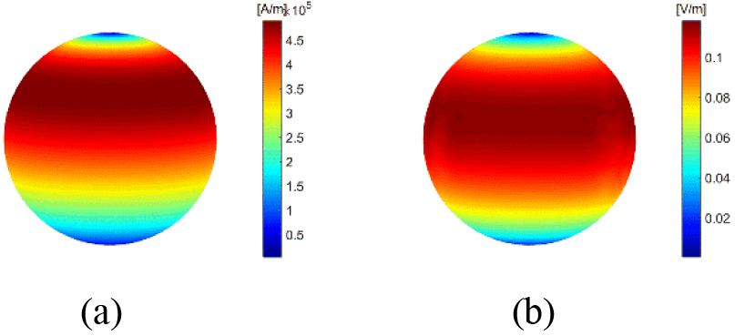
Figure 2: (a) Electric current density on the outer surface. (b) Magnetic current density on the outer surface.

The scattered fields in region $V_1$ along the line $\left(r=0.2\mathrm{m},0\le \theta \le \pi ,\varphi =\pi \mathrm{/}4\right)$ are shown in Figure 3. The total fields in the shell along the line $\left(r=0.315\mathrm{m},0\le \theta \le \pi ,\varphi =\pi \mathrm{/}4\right)$ are shown in Figure 4. The transmitted fields in the background media along the line $\left(r=1.2\mathrm{m},0\le \theta \le \pi ,\varphi =\pi \mathrm{/}4\right)$ are shown in Figure 5.

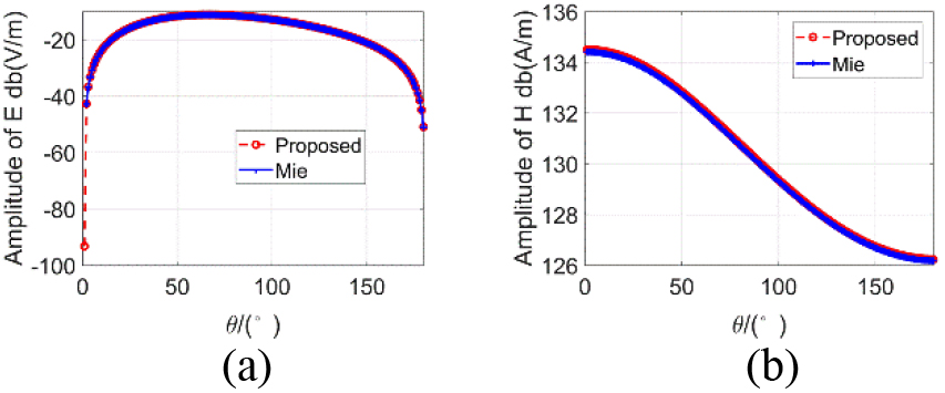
Figure 3: Scattered fields along the line ($r=0.2\mathrm{m}$, $0\le \theta \le \pi ,\varphi =\pi \mathrm{/}4$). (a) Electric field. (b) Magnetic field.

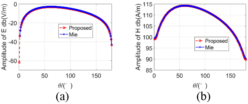
Figure 4: Total fields along the line ($r=0.315\mathrm{m}$, $0\le \theta \le \pi ,\varphi =\pi \mathrm{/}4$). (a) Electric field. (b) Magnetic field.

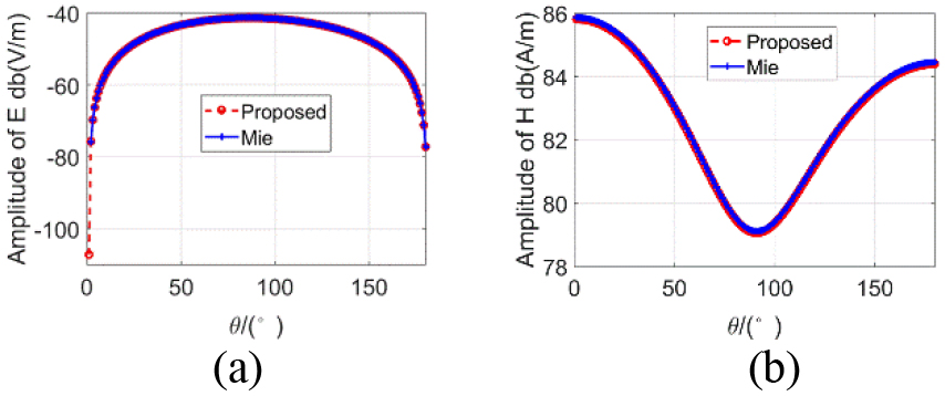
Figure 5: Transmitted fields along the line ($r=1.2\mathrm{m}$, $0\le \theta \le \pi ,\varphi =\pi \mathrm{/}4$). (a) Electric field. (b) Magnetic field.

The transmitted electric and magnetic fields on the XOZ plane in the region $-20\le z\le 20,1\le x\le 41,y=0$ are shown in Figures 6 and 7, respectively. The results calculated with proposed method agree well with reference results.

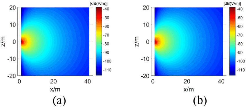
Figure 6: Transmitted fields on the XOZ plane. (a) Electric field calculated with the proposed method. (b) Electric field calculated with Mie series solution.

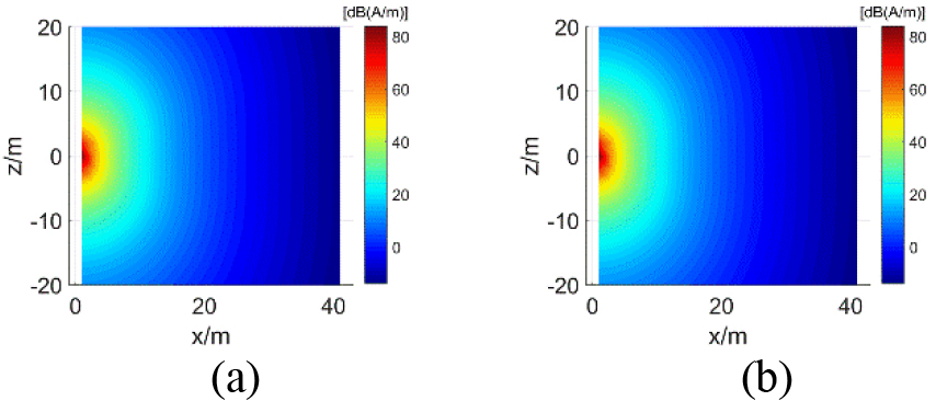
Figure 7: Transmitted fields on the XOZ plane. (a) Magnetic field calculated with the proposed method. (b) Magnetic field calculated with Mie series solution.

The transmitted fields of the spherical shell are also calculated at 50 Hz. The inner and outer surfaces of the shell are discretized into 8481 and 10212 RWG functions, respectively. The transmitted fields on the XOZ plane in the region $-20\le z\le 20,1\le x\le 41,y=0$ are shown in Figures 8 and 9, respectively. It is observed that the amplitude of transmitted fields at 50 Hz is attenuated to a very small level. The reason is that the thickness of the shell is about 13 times of the skin depth at 50 Hz while 0.6 times of the skin depth at 0.1 Hz.

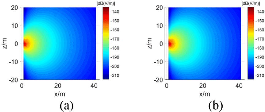
Figure 8: Transmitted fields on the XOZ plane. (a) Electric field calculated with the proposed method. (b) Electric field calculated with Mie series solution.

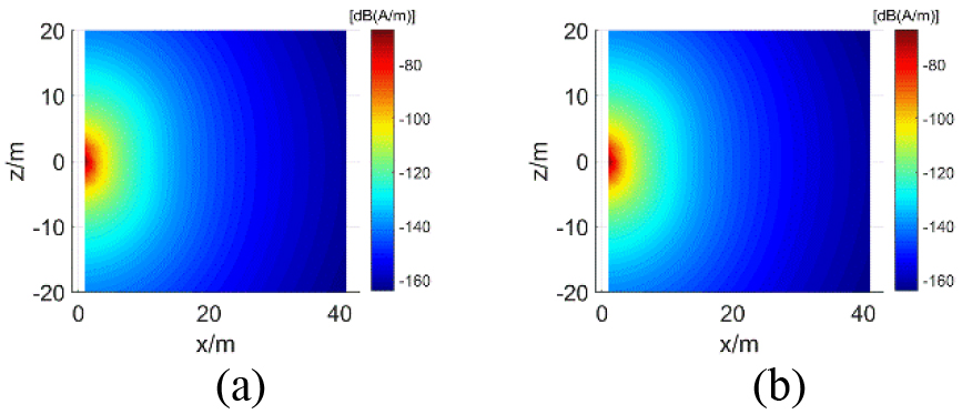
Figure 9: Transmitted fields on the XOZ plane. (a) Magnetic field calculated with the proposed method. (b) Magnetic field calculated with Mie series solution.

The proposed method can be easily extended to evaluate the transmitted fields of a source in a two-layered magnetic shell with large conductivity. We give the numerical results to verify the proposed method directly since the theory is similar. The inner and outer radii of the inner shell are $a=0.3\mathrm{m}$ and $b=0.33\mathrm{m}$, respectively. The inner and outer radii of the outer shell are $c=0.5\mathrm{m}$ and $d=0.53\mathrm{m}$, respectively. The regions $r<a$ and $b<r<c$ are free space. The parameters of shell $a<r<b$ and $c<r<d$ are ${\epsilon }_{r2}=1$, ${\mu }_{r2}=100$, and ${\sigma }_2=\mathrm{\hspace{0.33em}1.0}\times {10}^7\mathrm{S}\mathrm{/}\mathrm{m}$. The parameters of background region $d<r$ are ${\epsilon }_{r3}=81$, ${\mu }_{r3}=1$, and ${\sigma }_3=\mathrm{\hspace{0.33em}4}\mathrm{S}\mathrm{/}\mathrm{m}$. The frequency is 0.1 Hz. The inner and outer spherical surfaces of inner shell are discretized into 2556 and 3099 RWG functions, respectively. The corresponding total numbers of RWG functions on the inner and outer spherical surfaces of outer shell are 7032 and 7956, respectively. The electric current and magnetic current density on the surface $r=d$ are shown in Figure 10. Compared to Mie series solution, the relative errors of current densities are $-$49.6 and $-$41.9 dB, respectively.

The transmitted fields in the background media along the line $\left(r=1.2\mathrm{m},\mathrm{\hspace{0.17em}0}\le \theta \le \pi ,\varphi =\pi \mathrm{/}4\right)$ are shown in Figure 11. The transmitted electric and magnetic fields on the XOY plane in the region $-20\le x\le 20,1\le y\le 41,z=0$ are shown in Figures 12 and 13, respectively. They agree well with each other.

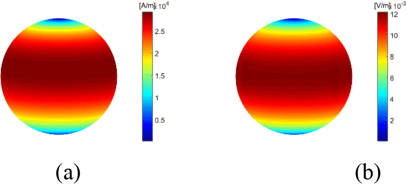
Figure 10: (a) Electric current density on the surface $r=d$. (b) Magnetic current density on the surface $r=d$.

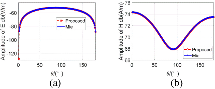
Figure 11: Transmitted fields along the line $\left(r=1.2\mathrm{m},0\le \theta \le \pi ,\varphi =\pi \mathrm{/}4\right)$. (a) Electric field. (b) Magnetic field.

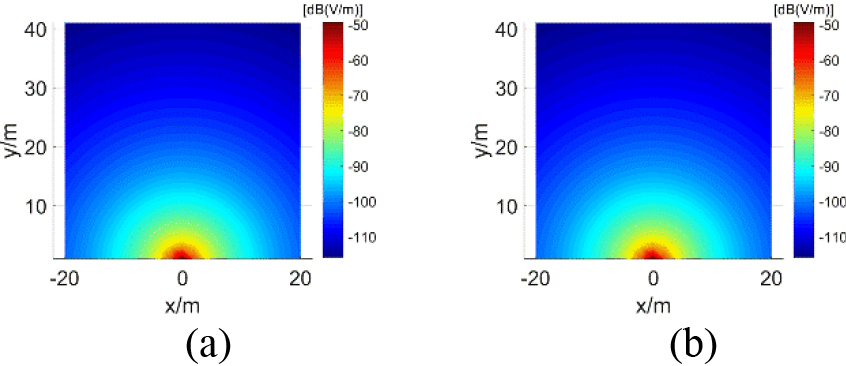
Figure 12: Transmitted fields on the XOY plane. (a) Electric field calculated with the proposed method. (b) Electric field calculated with Mie series solution.

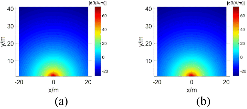
Figure 13: Transmitted fields on the XOY plane. (a) Magnetic field calculated with the proposed method. (b) Magnetic field calculated with Mie series solution.

IV. CONCLUSION

In this work, evaluation of the transmitted fields from a magnetic shell with large but finite conductivity at low frequencies is proposed. The shell is modeled as a penetrable object. EFIE in the exterior problem and MFIE in the interior problem for the shell are selected to capture the wave behaviors outside and inside the shell. Furthermore, loop-star decomposition is carried out on operators in the formulation to overcome the LFB problem. Appropriate rescaling coefficients are applied to the decomposed equation to improve the conditioning at low frequencies. Presented numerical results validate the accuracy of the proposed method.

ACKNOWLEDGMENT

This work was supported by the National Nature Science Foundation of China under Grant 62188102.

APPENDIX

A. Expressions of operators

The explicit expression of operators ${ℒ}_{iE}$, ${𝒦}_{iE}$, ${𝒦}_{iH}$, and ${ℒ}_{iH}$ in region $V_i$ are

$$\begin{array}{c}{ℒ}_{iE}\left\{\mathbf{X}\left({\mathbf{r}}^{\prime }\right)\right\}=-j{k}_i{\eta }_i{\int }_S{g}_i(\mathbf{r},{\mathbf{r}}^{\prime })\mathbf{X}\left({\mathbf{r}}^{\prime }\right)\mathit{d}{S}^{\prime }\hfill \\ +\frac{{\eta }_i}{j{k}_i}\nabla {\int }_S{g}_i(\mathbf{r},{\mathbf{r}}^{\prime }){\nabla }^{\prime }\cdot \mathbf{X}\left({\mathbf{r}}^{\prime }\right)\mathit{d}{S}^{\prime },\hfill \end{array}$$

(39)

$${𝒦}_{iE}\left\{\mathbf{X}\left({\mathbf{r}}^{\prime }\right)\right\}={\int }_S\nabla g_i(\mathbf{r},{\mathbf{r}}^{\prime })\times \mathbf{X}\left({\mathbf{r}}^{\prime }\right)\mathit{d}{S}^{\prime },$$

(40)

$${𝒦}_{iH}\left\{\mathbf{X}\left({\mathbf{r}}^{\prime }\right)\right\}={\int }_S\nabla g_i(\mathbf{r},{\mathbf{r}}^{\prime })\times \mathbf{X}\left({\mathbf{r}}^{\prime }\right)\mathit{d}{S}^{\prime },$$

(41)

$${ℒ}_{iH}\left\{\mathbf{X}\left({\mathbf{r}}^{\prime }\right)\right\}=\frac{1}{{\eta }_i^2}{ℒ}_{iE}\left\{\mathbf{X}\left({\mathbf{r}}^{\prime }\right)\right\}.$$

(42)

${𝒦}_{iE}$ and ${𝒦}_{iH}$ include both residue term and Cauchy principal value term. $k_i=\omega {\mu }_i{\epsilon }_{\mathrm{ieff}}$ and ${\eta }_i={\mu }_i\mathrm{/}{\epsilon }_{\mathrm{ieff}}$ are the wave number and wave impedance in region $V_i$, respectively. ${\epsilon }_{\mathrm{ieff}}={\epsilon }_i+{\sigma }_i\mathrm{/}j\omega$ is the effective permittivity in region $V_i$. $g_i(\mathbf{r},{\mathbf{r}}^{\prime })=e^{-j{k}_{i}R}\mathrm{/}4\pi R$ is the Green’s function in the region $V_i$.

B. Expressions of matrix entries in (14)

The expressions of matrix elements in (14) are as follows:

$$\begin{array}{c}{\mathbf{L}}_{iE}(m,n)=j{k}_i{\eta }_i{\int }_{S_m}{\mathbf{f}}_m\cdot {\int }_{S_n}{g}_i(\mathbf{r},{\mathbf{r}}^{\prime }){\mathbf{f}}_n\mathit{d}{r}^{\prime }\mathit{d}r\hfill \\ +\frac{{\eta }_i}{j{k}_i}{\int }_{S_m}\nabla \cdot {\mathbf{f}}_m\cdot {\int }_{S_n}{g}_i(\mathbf{r},{\mathbf{r}}^{\prime }){\nabla }^{\prime }\cdot {\mathbf{f}}_n\mathit{d}{r}^{\prime }\mathit{d}r,\hfill \end{array}$$

(43)

$${\mathbf{K}}_{iE}(m,n)={\int }_{S_m}\widehat{\mathbf{n}}\times {\mathbf{f}}_m\cdot {\int }_{S_n}\nabla g_i(\mathbf{r},{\mathbf{r}}^{\prime })\times {\mathbf{f}}_n\mathit{d}{r}^{\prime }\mathit{d}r,$$

(44)

$${\mathbf{K}}_{iH}(m,n)={\int }_{S_m}\widehat{\mathbf{n}}\times {\mathbf{f}}_m\cdot {\int }_{S_n}\nabla g_i(\mathbf{r},{\mathbf{r}}^{\prime })\times {\mathbf{f}}_n\mathit{d}{r}^{\prime }\mathit{d}r,$$

(45)

$$\begin{array}{c}{\mathbf{L}}_{2H}(m,n)=\frac{j{k}_i}{{\eta }_i}{\int }_{S_m}{\mathbf{f}}_m\cdot {\int }_{S_n}{g}_i(\mathbf{r},{\mathbf{r}}^{\prime }){\mathbf{f}}_n\mathit{d}{r}^{\prime }\mathit{d}r\hfill \\ +\frac{1}{j{k}_i{\eta }_i}{\int }_{S_m}\nabla \cdot {\mathbf{f}}_m\cdot {\int }_{S_n}{g}_i(\mathbf{r},{\mathbf{r}}^{\prime }){\nabla }^{\prime }\cdot {\mathbf{f}}_n\mathit{d}{r}^{\prime }\mathit{d}r,\hfill \end{array}$$

(46)

$${\mathbf{V}}_e^{\mathrm{in}}\left(m\right)={\int }_{S_m}{\mathbf{f}}_m\cdot {\mathbf{E}}^{\mathrm{in}}\mathit{d}\mathbf{r}.$$

(47)

REFERENCES

[1] M. A. Holloway, Z. Dilli, and N. Seekhao, and J. C. Rodgers “Study of basic effects of HPM pulses in digital CMOS integrated circuit inputs,” IEEE Trans. Electromagn. Compat., vol. 54, no. 5, pp. 1017-1027, Oct. 2012.

[2] H. Bagci. A. C. Yucel, J. S. Hesthaven, and E. Michielssen, “A fast Stroud-based collocation method for statistically characterizing EMI/EMC phenomena on complex platforms,” IEEE Trans. Magn., vol. 51, no. 2, pp. 301-311, May 2009.

[3] W. M. Rucker, R. Hoschek, and K. R. Richter, “Various BEM formulations for calculating eddy currents in terms of field variables,” IEEE Trans. Magn., vol. 31, no. 3, pp. 1336-1341, May 1995.

[4] D. Zheng, “Three-dimensional eddy current analysis by the boundary element method,” IEEE Trans. Magn., vol. 33, no. 2, pp. 1354-1357, Mar. 1997.

[5] B. Song, Z. Zhu, J. D. Rockway, and J. White, “A new surface integral formulation for wideband impedance extraction of 3-D structures,” 2003 IEEE/ACM International Conference on Computer Aided Design, San Jose, USA, Nov. 2003.

[6] Y.-H. Chu and W. C. Chew, “A robust surface-integral-equation formulation for conductive media,” Microw. Opt. Technol. Lett., vol. 46, no. 2, pp. 109-114, Jul. 2005.

[7] Z. G. Qian, W. C. Chew, and R. Suaya, “Generalized impedance boundary condition for conductor modeling in surface integral equation,” IEEE Trans. Microw. Theory Techn., vol. 55, no. 11, pp. 2354-2364, Nov. 2007.

[8] D. De Zutter and L. Knockaert, “Skin effect modeling based on a differential surface admittance operator,” IEEE Trans. Microw. Theory Tech., vol. 53, no. 8, pp. 2526-2538, Aug. 2005.

[9] T. L. Chhim, A. Merlini, L. Rahmouni, J. E. Ortiz Guzman, and F. P. Andriu, “Eddy current modeling in multiply connected regions via a full-wave solver based on the quasi-Helmholtz projectors,” IEEE Open J. Antennas Propag., vol. 1, pp. 534-548, 2020.

[10] T. Xia, H. Gan, M. Wei, W. C. Chew, H. Braunisch, Z. Qian, and K. Ay, “An integral equation modeling of lossy conductors with the enhanced augmented electric field integral equation,” IEEE Trans. Antennas Propag., vol. 65, no. 8, pp. 4181-4190, Aug. 2017.

[11] L. Zhang and M. S. Tong, “Low-frequency analysis of lossy interconnect structures based on two-region augmented volume-surface integral equations,” IEEE Trans. Antennas Propag. Early Access. doi: 10.1109/TAP.2021.3118849.

[12] S. Sharma and P. Triverio, “SLIM: A well-conditioned single-source boundary element method for modeling lossy conductors in layered media,” IEEE Antennas Wireless Propag. Lett., vol. 19, no. 12, pp. 2072-2076, Dec. 2020.

[13] M. Huynen, K. Y. Kapusuz, X. Sun, G. Van der Plas, E. Beyne, and D. Danir̈l, “Entire domain basis function expansion of the differential surface admittance for efficient broadband characterization of lossy interconnects,” IEEE Trans. Microw. Theory Techn., vol. 68, no. 4, pp. 1217-1233, Apr. 2020.

[14] S. Sharma and P. Triverio, “Electromagnetic Modeling of Lossy Materials with a Potential-Based Boundary Element Method,” IEEE Antennas Wireless Propag. Lett., Early Access. doi: 10.1109/LAWP.2021.3132626.

[15] S. M. Rao, D. R. Wilton, and A. W. Glisson, “Electromagnetic scattering by surfaces of arbitrary shape,” IEEE Trans. Antennas Propag., vol. 30, no. 3, pp. 409-418, May 1982.

[16] S. Y. Chen, W. C. Chew, J. M. Song, and J.-S. Zhao, “Analysis of low frequency scattering from penetrable scatterers,” IEEE Trans. Geosci. Remote Sens., vol. 39, no. 4, pp. 726-735, Apr. 2001.

[17] S. Yan, J. M. Jin, and Z. Nie, “EFIE analysis of low-Frequency problems with loop-star decomposition and Calder$\acute{\mathrm{o}}$n multiplicative preconditioner,” IEEE Trans. Antennas Propag., vol. 58, no. 3, pp. 857-867, Mar. 2010.

BIOGRAPHIES

Shifeng Huang received the B.S. and M.S. degrees from Wuhan University, Wuhan, China, in 2014 and 2017, respectively. He is currently working toward the Ph.D. degree in electronic engineering with Shanghai Jiao Tong University, Shanghai, China.

His current research interests include computational electromagnetics and its application in electromagnetic compatibility and scattering problems.

Gaobiao Xiao received the B.S. degree from the Huazhong University of Science and Technology, Wuhan, China, in 1988, the M.S. degree from the National University of Defense Technology, Changsha, China, in 1991, and the Ph.D. degree from Chiba University, Chiba, Japan, in 2002.

He has been a faculty member since 2004 with the Department of Electronic Engineering, Shanghai Jiao Tong University, Shanghai, China. His research interests are computational electromagnetics, coupled thermo-electromagnetic analysis, microwave filter designs, fiber-optic filter designs, phased array antennas, and inverse scattering problems.

Junfa Mao was born in 1965. He received the B.S. degree in radiation physics from the National University of Defense Technology, Changsha, China, in 1985, the M.S. degree in experimental nuclear physics from the Shanghai Institute of Nuclear Research, Chinese Academy of Sciences, Beijing, China, in 1988, and the Ph.D. degree in electronic engineering from Shanghai Jiao Tong University, Shanghai, China, in 1992.

Since 1992, he has been a Faculty Member with Shanghai Jiao Tong University. He was a Visiting Scholar with the Chinese University of Hong Kong, Hong Kong, from 1994 to 1995, and a Postdoctoral Researcher with the University of California at Berkeley, Berkeley, CA, USA, from 1995 to 1996. He has authored or coauthored more than 500 articles. His research interests include interconnect and package problems of integrated circuits and systems, and analysis and design of microwave components and circuits.

ACES JOURNAL, Vol. 37, No. 2, 238–245.
doi: 10.13052/2022.ACES.J.370213
© 2021 River Publishers

Abstract

I. INTRODUCTION

II. FORMULATION FOR THE SHELL

A. Equation formular at high frequency

B. Loop-star decomposition

III. NUMERICAL EXAMPLES

IV. CONCLUSION

ACKNOWLEDGMENT

APPENDIX

A. Expressions of operators

B. Expressions of matrix entries in (14)

REFERENCES

BIOGRAPHIES