Convolutional Neural Network for Coupling Matrix Extraction of Microwave Filters

Tarek Sallam^1,2 and Ahmed M. Attiya³

¹School of Applied Technology, Qujing Normal University, Qujing, Yunnan, PR China 655011

²Faculty of Engineering at Shoubra, Benha University, Cairo, Egypt
tarek.sallam@feng.bu.edu.eg

³Microwave Engineering Dept., Electronics Research Institute (ERI), Cairo, Egypt
attiya@eri.sci.eg

Submitted On: March 6, 2022; Accepted On: April 3, 2022

Abstract

Tuning a microwave filter is a challenging problem due to its complexity. Extracting coupling matrix from given S-parameters is essential for ?lter tuning and design. In this paper, a deep-learning-based neural network namely, a convolutional neural network (CNN) is proposed to extract coupling matrix from S-parameters of microwave filters. The training of the proposed CNN is based on a circuit model. In order to exhibit the robustness of the new technique, it is applied on 5- and 8-pole filters and compared with a shallow neural network namely, radial basis function neural network (RBFNN). The results reveal that the CNN can extract the coupling matrix of target S-parameters with high accuracy and speed.

Index Terms: convolutional neural network, coupling matrix, deep learning, microwave filters, parameters extraction.

1 INTRODUCTION

Microwave filters are widely used in all types of electronic systems [1, 2]. Tuning of microwave filter is an inevitable process in the design procedure of microwave filters. For the case of coupled resonator filter, extracting of the coupling matrix from the required S-parameters can be viewed as an inverse problem for microwavefilters.

Therefore, accurate solution of the inverse problem (extraction of coupling matrix) is crucial. However, it is extremely difficult to solve this inverse problem directly [3, 4]. Traditionally, the coupling matrix of the microwave filter is extracted by adopting the Cauchy method [5] or vector fitting [6]. However, these methods need to be repeated for many iterations in different conditions. Consequently, the process of filter design suffers from the time-consuming and complicated parameters extraction.

Neural network (NN) has been recognized as a powerful tool in microwave modeling and design[7–10]. Some conventional (shallow) NN techniques have been developed to extract the coupling matrix[11–13]. However, these techniques are not suitable for high-dimensional (many input variables) problems because data generation and model training become too complicated. A deep NN is applied to the parameter extraction of microwave filter [14]. However, there are too many layers in the deep NN, which make the training process complicated.

On the other hand, convolutional neural network (CNN) is a variant of deep network framework and achieves remarkable success on image and face recognition [15, 16]. Recently, it has gained much attention in the microwave field [17, 18]. It has unique capabilities of extracting underlying nonlinear features of input data. Two main advantages, sparse connectivity and shared weights, enable CNNs to have small numbers of parameters during learning and, hence, high training speed. Motivated by the inherent advantages of the CNN, it has been incorporated into coupling matrix extraction [19, 20].

In all the above NN methods, the training data is generated using full-wave electromagnetic (EM) model through simulation or measurement which becomes impractical when large training data is needed. Furthermore, the cost of training data generation increases exponentially with the number of input variables. Therefore, collection of training data using EM-based model to cover the interested input parameter range over a frequency band can be an overwhelmingly time-consuming task. Different from EM models, circuit models are used for all kinds of electronic designs. They are usually straightforward to build, and fast to evaluate.

In this paper, a CNN is used to extract the coupling matrix of ideal (target) S-parameters based on a circuit model. The CNN first extracts the features of S-parameters by using convolution layers and pooling layers, which are then mapped to the coupling matrix by full connection and output layers. To validate the effectiveness of the proposed CNN, it is applied on 5- and 8-pole microwave filters. The proposed CNN model is able to extract the coupling matrix of the ideal S-parameters with high accuracy and speed compared with a radial basis function neural network (RBFNN) [21–23] which is shallow (non-deep) NN.

2 CNN FOR CIRCUIT MODEL-BASED COUPLING MATRIX EXTRACTION

The circuit model-based equation that relates the coupling matrix M and filter S-parameters is given by [24]

$$S_{11}=1+2j{R}_1{\left[\gamma \mathbf{I}-j\mathbf{R}+\mathbf{M}\right]}_{11}^{-1}$$

$$S_{21}=-2j\sqrt{R_1{R}_2}{\left[\gamma \mathbf{I}-j\mathbf{R}+\mathbf{M}\right]}_{N1}^{-1},$$

(1)

where $\gamma$ = (f${\mathrm{0}}_{}$/BW)((f/f${\mathrm{0}}_{}$) – (f${\mathrm{0}}_{}$/f)), f, f${\mathrm{0}}_{}$, and BW are the frequency, filter center frequency, and filter bandwidth, respectively, N is the filter order, I is N $\mathrm{\times }$ N identity matrix, M is the N $\mathrm{\times }$ N symmetric coupling matrix, R is an N $\mathrm{\times }$ N matrix with all entries being zero except [R]${11}_{}$= R${\mathrm{1}}_{}$ and [R]${NN}_{}$= R${\mathrm{2}}_{}$, and R${\mathrm{1}}_{}$ and R${\mathrm{2}}_{}$ are the filter’s input and output coupling parameters, respectively, as shown in Fig. 1.

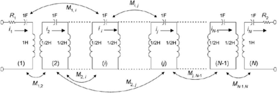
Figure 1: Equivalent circuit of an N-coupled resonator filter [24].

Figure 2 shows the CNN model for extracting the coupling matrix. The input to the CNN is the required vectors |S${\mathrm{11}}_{}$| and |S${\mathrm{21}}_{}$|, representing the scalar magnitudes of the two S-parameters at $ℛ$ frequency points in the required frequency range. Therefore, the total number of inputs is $2ℛ$. In the present case, the number of the frequency points $ℛ=2001$. The output of the CNN is the vector of nonzero coupling parameters M${\mathrm{n}\mathit{}\mathrm{z}}_{}$.

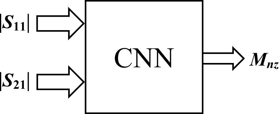
Figure 2: The circuit model-based CNN for coupling matrix extraction.

In order to generate the training and validation data of CNN, we assume a tolerance of $\pm$0.5 for every ideal nonzero coupling parameter. We then use 12,500 (10,000 for training and 2500 for validation) uniformly distributed random samples in this range for coupling parameters. For each sample of coupling parameters, eqn (1) is used to obtain the corresponding S-parameters. By swapping the data of coupling parameters and S-parameters, we can get the training and validation data for the coupling parameters extraction model. In the same way, the trained CNN is tested by the ideal set of S-parameters (corresponding to the ideal M${\mathrm{n}\mathit{}\mathrm{z}}_{}$ that is never used in the training), then the extracted M${\mathrm{n}\mathit{}\mathrm{z}}_{}$is compared to the ideal one.

3 THE PROPOSED CNN STRUCTURE

CNNs have one or more convolutional and pooling layers to learn the discriminative features from the input data. After all the convolutional and pooling layers, these learned features are then aggregated to the vectors by the fully connected (FC) layers for the regression task [25].

After many simulation trials, it is found that the CNN structure that provides the best accuracy is detailed in Table 1. First, the total 4002 inputs are reshaped into a 2 $\times$ 3 $\times$ 667 input image. Then, there are three convolutional (Conv) layers and three maximum pooling (MaxPool) layers. Each convolutional layer is followed by a pooling layer to reduce the dimension of network parameters. The first convolutional layer comprises eight feature maps. The number of feature maps at each convolutional layer is twice the previous layer, i.e., there are 16 and 32 feature maps in the second and third layers, respectively. The size of the feature map in each convolutional layer is fixed at 2 $\times$ 2. All convolutional layers have a stride of 1 and “same” padding. All pooling layers have a size of 2 $\times$ 2, stride 2, and “same” padding. After the sequence of convolutional and pooling layers, there is a single FC layer with 50 nodes followed by the output layer with a number of nodes equal to the number of nonzero coupling parameters. In order to avoid overfitting during training, a dropout operation with a rate of 50% is used at the end of the convolutional and pooling layers. The activation functions used in the convolutional layers and the FC layer are rectified linear unit (ReLU) and exponential linear unit (ELU), respectively. Since this is a regression problem instead of a classification problem, no activation is used at the output layer (linear activation).

4 EXAMPLES

To verify the performance of the CNN-based coupling matrix extraction, it is applied on 5- and 8-pole microwave filters. The Adam (adaptive momentum) optimization algorithm [26] is used to update the network weights and the loss function used for this network is the mean squared error. The initial value of the learning rate is 0.001. During the training, the learning rate is decreased by a rate of 0.1 each 40% of number of epochs. The batch size is 40 and number of epochs is 10. To further verify the performance of the CNN, it is compared to that of the RBFNN. Both NNs have the same number of inputs (4002) and outputs (Length$\{$M${\mathrm{n}\mathit{}\mathrm{z}}_{}$$\mathrm{\}}$) as well as the same size of training and validation datasets (10,000 and 2500, respectively). In all examples, the filter’s input and output coupling parameters are assumed to be equal, i.e., R${\mathrm{1}}_{}$ = R${\mathrm{2}}_{}$.

Table 1: The proposed CNN structure

Layer	Size	Nodes	Stride	Padding	Activation
Input (image)	–	(2$\times$3$\times$667) = 4002	–	–	–
Conv1	2$\times$2	8	1	Same	ReLU
MaxPool1	–	2	–
Conv2	16	1	ReLU
MaxPool2	–	2	–
Conv3	32	1	ReLU
MaxPool3	–	2	–
50% Dropout
FC	–	50	–	–	ELU
Output	–	Length{M${\mathrm{n}\mathit{}\mathrm{z}}_{}$}	–	–	Linear

4.1 5-Pole filter

In this example, we use the proposed CNN to develop a parameter-extraction model for a 5-pole dielectric resonator filter with a 3.4-GHz center frequency and a 54-MHz bandwidth [24]. The nonzero coupling parameters are M${\mathrm{n}\mathit{}\mathrm{z}}_{}$ = [R${\mathrm{1}}_{}$ M${\mathrm{12}}_{}$ M${\mathrm{14}}_{}$ M${\mathrm{23}}_{}$ M${\mathrm{34}}_{}$ M${\mathrm{45}}_{}$]$T^{}$with their ideal values shown in Table 2. Table 2 also shows the extracted coupling values by RBFNN and CNN. It can be seen that the values of CNN are much closer to the ideal ones than those of RBFNN. The used shallow RBFNN has only one hidden layer with 300 neurons and cannot represent this high-dimensional input–output relationship effectively. Our proposed CNN modeling technique is suitable for this high-dimensional modeling problem.

Figure 3 shows the S-parameters corresponding to the coupling values in Table 2. As can be seen, there is a perfect agreement between the responses from the ideal and extracted coupling matrix of CNN compared with RBFNN, that is, owing to the capability of CNN to extract the hidden features in the input data, S-parameters, automatically. On the other hand, because the RBFNN is shallow, it cannot strengthen the network training process by reconstructing the input S-parameters.

Table 2: The ideal and extracted coupling values by RBFNN and CNN for a 5-pole filter

M${\mathrm{n}\mathit{}\mathrm{z}}_{}$	RBFNN	CNN	Ideal
R${\mathrm{1}}_{}$	1.1098	1.1345	1.1330
M${\mathrm{12}}_{}$	0.8138	0.8659	0.8660
M${\mathrm{14}}_{}$	$-$0.1450	$-$0.2525	$-$0.2520
M${\mathrm{23}}_{}$	0.7389	0.7942	0.7920
M${\mathrm{34}}_{}$	0.5287	0.5946	0.5950
M${\mathrm{45}}_{}$	0.8594	0.9006	0.9010

4.2 8-Pole filter

The second example involves the parameter-extraction of an 8-pole elliptic-function filter with 30-MHz bandwidth centered at 3 GHz [27]. The nonzero couplings are R${\mathrm{1}}_{}$, M${\mathrm{12}}_{}$, M${\mathrm{23}}_{}$, M${\mathrm{27}}_{}$, M${\mathrm{34}}_{}$, M${\mathrm{36}}_{}$, M${\mathrm{45}}_{}$, M${\mathrm{56}}_{}$, M${\mathrm{67}}_{}$, and M${\mathrm{78}}_{}$. However, the coupling matrix of this filter is dual-symmetrical meaning that it is symmetrical w.r.t. its anti-diagonal as well as its diagonal [28]. Therefore, M${\mathrm{12}}_{}$= M${\mathrm{78}}_{}$, M${\mathrm{23}}_{}$= M${\mathrm{67}}_{}$, and M${\mathrm{34}}_{}$ = M${\mathrm{56}}_{}$. Consequently, the output of NNs is M${\mathrm{n}\mathit{}\mathrm{z}}_{}$ = [R${\mathrm{1}}_{}$ M${\mathrm{12}}_{}$ M${\mathrm{23}}_{}$ M${\mathrm{27}}_{}$ M${\mathrm{34}}_{}$ M${\mathrm{36}}_{}$M${\mathrm{45}}_{}$]$T^{}$. Table 3 shows the ideal as well as the extracted coupling values by both NNs with their corresponding S-parameters shown in Fig. 4.

Table 3: The ideal and extracted coupling values by RBFNN and CNN for 8-pole filter

M${\mathrm{n}\mathit{}\mathrm{z}}_{}$	RBFNN	CNN	Ideal
R${\mathrm{1}}_{}$	1.2206	1.2415	1.2420
M${\mathrm{12}}_{}$	0.8977	0.9387	0.9380
M${\mathrm{23}}_{}$	0.5882	0.6300	0.6310
M${\mathrm{27}}_{}$	$-$0.0110	$-$0.0172	$-$0.0180
M${\mathrm{34}}_{}$	0.5313	0.5729	0.5760
M${\mathrm{36}}_{}$	0.0034	0.0637	0.0660
M${\mathrm{45}}_{}$	0.4549	0.5193	0.5190

According to Table 3 and Fig. 4, a very good match between the ideal and extracted coupling parameters by CNN along with an excellent agreement between the responses from the ideal and extracted coupling matrix by CNN have been achieved, compared to RBFNN. This again proves that the CNN is much more accurate than the RBFNN for coupling matrixextraction.

Table 4: Percentage RMSE and training time of RBFNN and CNN for 5- and 8-pole filters

NN	5-Pole filter	8-Pole filter
	Training Time	RMSE (%)	Training Time	RMSE (%)
CNN	39 s	0.1413	38 s	0.2260
RBFNN	19.6 min	7.7997	17.7 min	6.3894

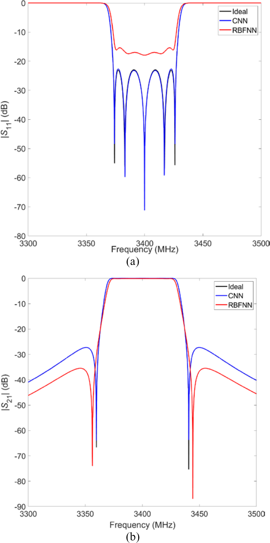
Figure 3: The responses calculated by the coupling values in Table 2: (a) Return loss and (b) insertion loss.

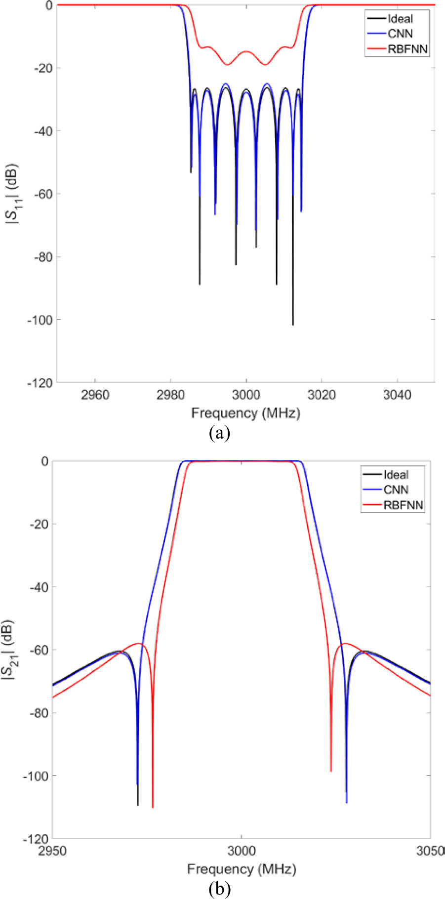
Figure 4: The responses calculated by the coupling values in Table 3: (a) Return loss and (b) insertion loss.

Table 4 shows the training time as well as the percentage root mean square error (RMSE) between ideal and extracted couplings by NNs for 5- and 8-pole filters. It can be seen that the CNN modeling for the extraction of coupling matrix is with much higher accuracy and shorter training time than the RBFNN modeling.

Moreover, our proposed circuit model-based CNN can provide parameter-extraction solutions instantly, while the full-wave EM model-based methods can take hours to extract the solutions by repetitively simulating/measuring the filter during optimization iterations.

5 CONCLUSION

A circuit model-based CNN is proposed to extract coupling matrix from S-parameters. The results show that the proposed CNN method can be used reliably to perform the parameter extraction for microwave filters. Compared to the shallow NN, the deep-learning-based CNN is much more accurate and faster in extracting the coupling parameters. Unlike the full-wave EM model-based methods, our proposed CNN model does not need to simulate and/or measure the filter iteratively. Once the CNN model is developed, it can be used to quickly extract the coupling parameters of microwave filters.

REFERENCES

[1] R. J. Cameron, C. M. Kudsia, and R. T. Mansour, Microwave Filters for Systems: Fundamentals, Design and Applications. Hoboken, NJ, USA, Wiley, 2018.

[2] S. Saleh, W. Ismail, I. S. Z. Abidin, and M. H. Jamaluddin, “Compact 5G Hairpin bandpass filter using non-uniform transmission lines theory,” Applied Computational Electromagnetic Society (ACES) Journal, vol. 36, no. 2, pp. 126-131, Feb. 2021.

[3] L. Accatino, “Computer-aided tuning of microwave filters,” in IEEE MTT-S Int. Microw. Symp. Dig., pp. 249-252, Jun. 1986.

[4] M. Yu and W. C. Tang, “A fully automated filter tuning robots for wireless base station diplexers,” in Proc. Workshop, Comput. Aided Filter Tuning, IEEE Int. Microw. Symp., Philadelphia, PA, USA, pp. 8-13, Jun. 2003.

[5] G. Macchiarella and D. Traina, “A formulation of the Cauchy method suitable for the synthesis of lossless circuit models of microwave filters from Lossy measurements,” IEEE Microw. Wireless Compon. Lett., vol. 16, no. 5, pp. 243-245, May 2006.

[6] C.-K. Liao, C.-Y. Chang, and J. Lin, “A vector-fitting formulation for parameter extraction of lossy microwave filters,” IEEE Microw. Wireless Compon. Lett., vol. 17, no. 4, pp. 277-279, Apr. 2007.

[7] Q.-J. Zhang, K. C. Gupta, and V. K. Devabhaktuni, “Artificial neural networks for RF and microwave design-From theory to practice,” IEEE Trans. Microw. Theory Techn., vol. 51, no. 4, pp. 1339-1350, Apr. 2003.

[8] H. Kabir, L. Zhang, M. Yu, P. H. Aaen, J. Wood, and Q.-J. Zhang, “Smart modeling of microwave devices,” IEEE Microw. Mag., vol. 11, no. 3, pp. 105-118, May 2010.

[9] Z. S. Tabatabaeian and M. H. Neshati, “Design investigation of an X-band SIW H-plane band pass filter with improved stop band using neural network optimization,” Applied Computational Electromagnetic Society (ACES) Journal, vol. 30, no. 10, pp. 1083-1088, Aug. 2021.

[10] Z. S. Tabatabaeian and M. H. Neshati, “Development of a low profile and wideband backward-wave directional coupler using neural network,” Applied Computational Electromagnetic Society (ACES) Journal, vol. 31, no. 12, pp. 1404-1409, Aug. 2021.

[11] H. Kabir, Y. Wang, M. Yu, and Q. J. Zhang, “High dimensional neural network techniques and applications to microwave filter modeling,” IEEE Trans. Microwave Theory Tech., vol. 58, no. 1, pp. 145-156, Jan. 2010.

[12] C. Zhang, J. Jin, W. Na, Q. -J. Zhang, and M. Yu, “Multivalued neural network inverse modeling and applications to microwave filters,” IEEE Trans. Microwave Theory Tech., vol. 66, no. 8, pp. 3781-3797, Aug. 2018.

[13] J. -J. Sun, X. Yu, and S. Sun, “Coupling matrix extraction for microwave filter design using neural networks,” 2018 IEEE International Conference on Computational Electromagnetics (ICCEM), pp. 1-2, 2018.

[14] J. Jin, F. Feng, W. Zhang, J. Zhang, Z. Zhao, and Q. -J. Zhang, “Recent advances in deep neural network technique for high-dimensional microwave modeling,” 2020 IEEE MTT-S International Conference on Numerical Electromagnetic and Multiphysics Modeling and Optimization (NEMO), pp. 1-3, 2020.

[15] J. Fu, H. Zheng, and T. Mei, “Look closer to see better: recurrent attention convolutional neural network for fine-grained image recognition,” IEEE Conference on Computer Vision and Pattern Recognition (CVPR), Honolulu, HI, USA, pp. 4476-4484, Jul. 2017.

[16] T. H. Kim, C. Yu, and S. W. Lee, “Facial expression recognition using feature additive pooling and progressive fine-tuning of CNN,” Electron. Lett., vol. 54, no. 23, pp. 1326-1327, 2018.

[17] Y. Wang, Z. Zhang, Y. Yi, and Y. Zhang, “Accurate microwave filter design based on particle swarm optimization and one-dimensional convolution autoencoders,” Int J RF Microw Comput Aided Eng., vol. 32, no. 4, 2022.

[18] H. Arab, I. Ghaffari, L. Chioukh, S. O. Tatu, and S. Dufour, “A Convolutional neural network for human motion recognition and classification using a millimeter-wave doppler radar,” IEEE Sensors Journal, vol. 22, no. 5, pp. 4494-4502, Mar. 2022.

[19] J. J. Sun, S. Sun, X. Yu, Y. P. Chen, and J. Hu, “A deep neural network based tuning technique of lossy microwave coupled resonator filters,” Microw. Opt. Technol. Lett., vol. 61, no. 9, pp. 2169-2173, 2019.

[20] Y. Zhang, Y. Wang, Y. Yi, J. Wang, J. Liu, andZ. Chen, “Coupling matrix extraction of microwave filters by using one-dimensional convolutional autoencoders,” Front. Phys., vol. 9, Nov. 2021.

[21] T. Sallam, A. B. Abdel-Rahman, M. Alghoniemy, Z. Kawasaki, and T. Ushio, “A Neural-network-based beamformer for phased array weather radar,” IEEE Transactions on Geoscience and Remote Sensing, vol. 54, no. 9, pp. 5095-5104, Sept. 2016.

[22] T. Sallam, A. B. Abdel-Rahman, M. Alghoniemy, and Z. Kawasaki, “A novel approach to the recovery of aperture distribution of phased arrays with single RF channel using neural networks,” 2014 Asia-Pacific Microwave Conference, Sendai, Japan, pp. 879-881, 2014.

[23] X. Jia, Q. Ouyang, T. Zhang, and X. Zhang, “A novel adaptive tracking algorithm for the resonant frequency of EMATs in high temperature,” Applied Computational Electromagnetic Society (ACES) Journal, vol. 33, no. 11, pp. 1243-1249, Jul. 2021.

[24] M. A. Ismail, D. Smith, A. Panariello, Y. Wang, and M. Yu, “EM-based design of large-scale dielectric-resonator filters and multiplexers by space mapping,” IEEE Trans. Microw. Theory Tech., vol. 52, no. 1, pp. 386-392, Jan. 2004.

[25] T. Sallam and A. M. Attiya, “Convolutional neural network for 2D adaptive beamforming of phased array antennas with robustness to array imperfections,” International Journal of Microwave and Wireless Technologies, vol. 13, no. 10, pp. 1096-1102, Dec. 2021.

[26] D. P. Kingma and J. Ba, “Adam: a method for stochastic optimization,” Proc. of the 3rd Int. Conf. on Learning Representations (ICLR), San Diego, CA, USA, 2015.

[27] H.-T. Hsu, Z. Zhang, K. A. Zaki, and A. E. Ati, “Parameter extraction for symmetric coupled-resonator filters,” IEEE Trans. Microw. Theory Techn., vol. 50, no. 12, pp. 2971-2978, Dec. 2002.

[28] J. W. Bandler, S. H. Chen, and S. Daijavad, “Exact sensitivity analysis for the optimization of coupled cavity filters,” J. Circuit Theory Applicat., vol. 31, pp. 63-77, 1986.

BIOGRAPHIES

Tarek Sallam was born in Cairo, Egypt, in 1982. He received the B.S. degree in electronics and telecommunications engineering and the M.S. degree in engineering mathematics from Benha University, Cairo, Egypt, in 2004 and 2011, respectively, and the Ph.D. degree in electronics and communications engineering from Egypt-Japan University of Science and Technology (E-JUST), Alexandria, Egypt, in 2015. In 2006, he joined the Faculty of Engineering at Shoubra, Benha University. In 2019, he joined the Faculty of Electronic and Information Engineering, Huaiyin Institute of Technology, Huai’an, Jiangsu, China. In 2022, he joined the School of Applied Technology, Qujing Normal University, Qujing, Yunnan, China, where he is currently an Associate Professor. He was a Visiting Researcher with the Electromagnetic Compatibility Lab, Osaka University, Osaka, Japan, from August 2014 to May 2015. His research interests include evolutionary optimization, neural networks and deep learning, phased array antennas with array signal processing and adaptivebeamforming.

Ahmed M. Attiya received the M.Sc. and Ph.D. degrees in electronics and electrical communications from the Faculty of Engineering, Cairo University, Cairo, Egypt, in 1996 and 2001, respectively. He joined the Electronics Research Institute as a Researcher Assistant in 1991. In the period from 2002 to 2004, he was a Postdoc with the Bradley Department of Electrical and Computer Engineering, Virginia Tech. In the period from 2004 to 2005, he was a Visiting Scholar with Electrical Engineering Department, University of Mississippi. In the period from 2008 to 2012, he was a Visiting Teaching Member with King Saud University. He is currently a Full Professor and the Head of Microwave Engineering Department, Electronics Research Institute. He is also the Founder of Nanotechnology Lab., Electronics Research Institute.

ACES JOURNAL, Vol. 37, No. 7, 805–810.
doi: 10.13052/2022.ACES.J.370707
© 2022 River Publishers

Abstract

1 INTRODUCTION

2 CNN FOR CIRCUIT MODEL-BASED COUPLING MATRIX EXTRACTION

3 THE PROPOSED CNN STRUCTURE

4 EXAMPLES

4.1 5-Pole filter

4.2 8-Pole filter

5 CONCLUSION

REFERENCES

BIOGRAPHIES