A Difference Subgridding Method for Solving Multiscale Electro-Thermal Problems
Xiaoyan Zhang, Ruilong Chen, and Aiyun Zhan
1School of Information Engineering, East China Jiaotong University, Nanchang 330013, China
xy_zhang3129@ecjtu.edu.cn, 2465246593@qq.com, 707290432@qq.com
Submitted On: January 13, 2021; Accepted On: February 20, 2022
Abstract
Because of less memory costs and time consumption, a finite difference subgrid technique can effectively deal with multiscale problems in electromagnetic fields. When used in Maxwell equation, symmetric elements of the matrix are required; otherwise, the algorithm will be unstable. Usually, the electro-thermal problem also contains multiscale structures. However, the coefficient matrix of the heat transfer equation is asymmetric because the parameters of the equation vary with temperature and the Robbin boundary condition is used as well. In this paper, a three-dimensional (3D) finite difference subgridding method is proposed to simulate the electro-thermal coupling process of the multiscale circuits. The stability condition of the algorithm is deduced with a matrix method. And the efficiency and the effectiveness of the proposed subgridding approach are verified through square- and n-shaped resistances. Compared with the results of the COMSOL software and the traditional finite difference method (FDM), the proposed subgridding method has less unknowns and faster speed.
Keywords: Electro-thermal problems, finite-difference method (FDM), multiscale, subgridding method.
I. INTRODUCTION
With the increase of the integration of the electronic components, Joule heat of the circuits becomes a severe problem; sometimes, it will lead to the decline of the reliability of the circuit [1, 2]. In order to solve this problem, the variation of the electromagnetic component parameters with the temperature [1–4], the distribution of the temperature in the circuit [5–7], and the influence of the high temperature on circuit performance [1, 2, 8] arouse the researchers’ study interests to guide circuit design and improve its stability. The difficulty of this study is that the electricity is the cause of the Joule heat, and the heat will affect the electrical parameters in return. They are coupled with each other.
Using the commercial software COMSOL to establish an electro-thermal model is one of the effective methods to solve this issue [9, 10]. However, the COMSOL is based on a finite-element method (FEM); so it has the shortcomings of low efficiency and heavy calculation burden in commutating the transient temperature field [11].
In the last decades, some algorithms have been further developed and used to study the variation of the circuit’s temperature and its effects on the device performance. In 2005, the heat transfer equation was analytically solved to evaluate the changes of temperature and thermal resistance of a microwave power field effect transistor (FET) unit [3]. However, the analytical method is only suitable for solving the electro-thermal problems of some specific structures. In 2008, a semi-analytical method was proposed based on the assumption that the substrate is half infinite. The method was applied to observe the nonlinear characteristics of an integrated resistance by considering the changes of the electrical conductivity () and the thermal conductivity () with temperature [4]. Due to the limitation of the analytical method, this approach is not suitable for modeling a model of finite substrate. In 2011, a numerical method of a finite-volume method (FVM) was presented and applied to estimate the temperature distribution profile of a three-dimensional (3D) power delivery network (PDN) package [1]. Only the variation of with temperature is considered. In 2016, our group developed a two-dimensional (2D) radial point interpolation method (RPIM) for electro-thermal coupling modeling. Although the temperature variation of the and were taken into account, the instability of the 3D meshless method of the RPIM still needs to be solved [5]. In 2018, a finite difference time domain method (FDTD) and a volume-element method (VEM) were combined for the transient analysis of gas-insulated transmission lines’ (GILs) electro-thermal performance [6]. Similarly, the change of resistance with temperature is introduced into the modeling process. In 2019, a 3D RPIM was presented to study the temperature response from a through-silicon via (TSV). And the effects of the , , and the specific heat C were taken into account [7]. Whereas, the problem of meshless algorithm, which we mentioned earlier, still needs to be faced. In 2020, the finite difference method (FDM) was introduced into a SPICE simulation tool for observing the characteristics of an insulated gate bipolar transistor (IGBT) at different temperatures. The charge motion of the semiconductor materials was introduced into the voltage equations [8].
Among the above algorithms, the FDM has the advantages of numerical stability and relatively simple implementation; so it is widely used in temperature field modeling [6, 8, 12]. One of the disadvantages of the FDM is difficulty in dealing with multiscale problems. Because the uniformly fine mesh of the FDM will result in a very large memory cost and the extension of the iterations. To solve this issue, some subgridding algorithms, such as a variable step size method (VSSM) [13], a spatial subgridding algorithm with separated temporal and spatial interfaces [14], a hybrid implicit–explicit FDTD method (HIE-FDTD) [15], and a Huygens subgridding FDTD method [16] were proposed and successfully applied in solving Maxwell equations. Since at least two sizes of grids are applied to the subgridding algorithm and the time steps of the domains with different grid sizes can be different, the simulations of the coarse grid and the fine grid can be carried out separately. In this way, the subgridding method can reduce the number of the unknowns and shorten the simulation time. Unfortunately, the data on the grids’ boundary needs to be obtained by the interpolation approach, which will destroy the symmetry of the algorithm. In order to ensure the stability of the subgridding approach, an effective solution is to make the element distribution of its coefficient matrix symmetrical [17], but it is difficult in mathematics; another simpler way is to derive the stability conditions of the algorithm so that it can run under certain conditions [18].
Usually, multiscale structures are often included in a circuit. Especially, for solving such an electro-thermal problem, electrical insulation and thermal radiation boundary conditions exist. In addition, the values of the electrical conductivity and the thermal conductivity of the circuit are related to the temperature. All these lead to an asymmetric coefficient matrix of the subgridding algorithm.
In this paper, a finite difference subgridding method for modeling the coupled electro-thermal equations is presented. In the subgridding scheme, the iterations in coarse grid and fine grid are performed respectively; and the spatial and the temporal linear interpolations are applied to obtain the values on the boundary surface. A matrix method [18] is introduced to derive the stability condition of the algorithm. In each march-on-in-time process, the coefficient matrix of the algorithm is updated as and change. And the and will vary with the temperature . To validate the efficiency of the proposed method, the transient temperature distributions of a square and an n-shaped copper resistances are simulated and compared with the results of the commercial software COMSOL and the traditional FDM, which demonstrate its effectiveness and efficiency.
This paper is arranged in the following manner. In Section II, theories and mathematics of the proposed method for the 3D electro-thermal problems as well as the stability condition are derived. In Section III, the numerical results are compared with those of the COMSOL software and the traditional FDM. In Section IV, conclusion is drawn.
II. THEORIES AND NUMERICAL METHODS
A. The coupled electro-thermal equations
A multiscale structure as shown in Figure 1 is considered in this research. In this model, a copper resistor with a smaller size of is integrated on a cuboid silicon substrate (). This device is assumed to be physically small. And because the speed of thermal change is far less than the speed of the electromagnetic field transmission, the electromagnetic field on the resistance is regarded as a static field. Therefore, the problem of the electro-thermal mutual coupling can be regarded as an electrostatic field producing Joule heat losses of P, and then the P becomes the thermal source and leads to heat conduction. In turn, the spatial distributions of the temperature will change the parameters of thedevice.
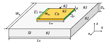
Figure 1: Electro-thermal model of a resistor.
This physical mechanism can be described by the following mathematical equation:
| (1) |
where the constants and C represent a density and a specific heat capacity of a material, respectively, K stands for the material’s thermal conductivity, is the temperature, and t represents the time. The power density P is calculated by
| (2) |
Here, represents the copper’s electric potential, and it is estimated by
| (3) |
d is the height of the copper. Its conductivity is defined as
| (4) |
where is an electrical resistivity and represents a temperature coefficient.
As Figure 1 shows, the positive electrode () of the copper is impinged on an U voltage and its negative electrode () is grounded (i.e., Dirichlet boundary or first-type boundary). In addition, the electrical insulation (Neumann boundary or second-type boundary) at , the thermal radiation (the third-type boundary or Robbin boundary) at boundary , and the other edges of the circuit that are cooled to are supposed. These conditions are expressed as
| (5a) |
and
| (5b) |
where is the norm of the boundary, h is the convective heat transfer coefficient, and is the ambient temperature. The empirical formula for can be found in [4].
B. Application of the finite difference subgridding method to the coupled electro-thermal equations
In this electro-thermal model, only copper is partitioned with a uniform fine grid of , while the substrate is divided by a uniform coarse grid of . Therefore, when calculating , there is only one kind of grid in the computational domain. After using the central difference method to eqn (3) to estimate its derivatives, at the fine cell (i, j) can be estimated by
| (6) |
where , (p=1, 2. q=i, j), .
On Neumann boundary of eqn (5a), eqn (6) becomes
| (7) |
Then, the Joule heat losses of P is
| (8) |
Whereas, there are two grid sizes on the Si substrate. To describe the subgridding algorithm clearly, the FDM of the temperature field on an upper left corner of the top surface in Figure 1 is cut out to be discussed in detail. This is typical because the grids on the top surface are constrained by the third-type boundary condition.
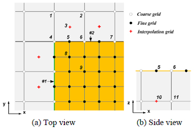
Figure 2: An interface of the coarse grids and subgrids on an upper left corner of the top surface.
The key of a subgridding method is the field coupling between the coarse mesh and the fine mesh. In this paper, the coupling is realized by linear interpolation. For simplicity and illustration purpose, the 2:1 ratio of the coarse cell and the fine cell is used as Figure 2. The coarse grid borders the fine grid. There are three types of grids: coarse grid, fine grid, and interpolation grid.
The cells “1, 2, 4, 6, 7” in Figure 2(a) and “11” in Figure 2(b) are coarse grids, where “6, 7” on the subgridding interface; the “5, 8, 9” are fine grids, where “5” on the interface, and the point “3, 10” is extra added to estimate its value. All the unknown temperature fields in Figure 2(a) are constrained by the Robbin boundary conditions of eqn (5b). Besides, the temperature fields of the other grids in the substrate, such as “11,” have no constraints.
Similarly, the T of these grids, except for “3, 10,” can be obtained by applying the FDM approach. After some manipulations, their formulas can be written as
| (9) |
where P = 0. But for the grids in the copper area, P is calculated by eqn (8); n is the iteration time step, and the time step ratio m is also the ratio of the spatial step, which is defined by
| (10) |
The = (, , , , ), (, , , , ), where
| (11) |
Here, , =c or f; p=1, 2, q=i, j, k; .
For the grids in different regions, m, , and are different.
For the grid “1, 2, 4, 6, 7,” m=1, = c, (, ,), where , ; (,,).
For the grid “5, 8, 9,” m is defined by eqn (10), and = f, , and are the same as above; in particular, T is interpolated by
| (12) |
and is introduced to estimate T. T is also introduced to estimate T, which is interpolated by the two adjacent coarse grids along x-axis.
For the grid “11,” m = 1, = c, (,), (, ) .
Since “6” is located on the boundary of the grid, when calculating T, T should be known at the same time. However, “9” is located on a fine cell. Due to the different time steps between the fine grid and the coarse grid, T needs to be iterated m times to reach the same time as T. Therefore, the two grids are coupled with each other.
To facilitate understanding, suppose that the current time step is n and all the fields are known. We summarize the update process of the proposed subgridding scheme into the following steps.
Step #1: Compute the electric potential equations of eqn (6)–(8) to obtain the Joule heat losses of P.
Step #2: Compute eqn (9) with to update , , and of the coarse grid and , , and of the interface grid to be , , , , , and . Then, compute eqn (12) to obtain and , , and . Similarly, eqn (9) with is executed to calculate , , and of the fine grid. Take as an example:
| (13) | |
Step #3: Update the temperature fields of the fine grids from the time step n+1/m to n+2/m. It should be noted that in order to obtain , , and needs to be interpolated in advance through and , and . This process will be repeated until the time step increases to n+1. Take as an example:
| (14) | |
where .
Step #4: Renew both and K with the temperatures calculated in Step #2 and Step #3. Go to Step #1.
C. Stability analysis
The explicit equation of (9) is conditionally stable. In this paper, the fine cell’s time step is first derived to be by using the matrix method, and then is determined by using the same method and considering the relationship with at the same time. Finally, is updated to 1/m times of as eqn (10).
Specifically, the source-free form of eqn (9) is arranged into the following equation:
| (15) |
where
| (16) |
where
A necessary condition for is that when , the spectral radius of the coefficient matrix must satisfy
| (17) |
where , and and represent the eigenvalue element of
From eqn (17), we have
| (18) |
By applying the same method, can be preliminarily determined. In this case, only
| (19) |
Therefore, can be updated to
| (20) |
in turn.
Theoretically, will change with T, but this change is negligible and can be ignored. To reduce the time loss, a fixed time step is used in the program execution.
III. NUMERICAL EXPERIMENTS
A. Cuboid resistor integrated on a Si substrate
The main parameters of Figure 1 are listed in Table 1. The parameters of and K can be found in [4]. A square wave signal with a voltage of 5 V is impinged on the resistor. The voltage period is 0.08 s. m sets to 4 in this experiment.
Table 1: Parameters of Figure 1
| L,W,d | 20,20,0.01 mm | T= T | 20 |
| L,W,D | 40,40,20 mm | h | 24 W/mK |
| 2.329 g/cm | C | 700 J/kgK | |
| 2.5 mm | U | 5 V | |
| 0.004 s | m | 4 |
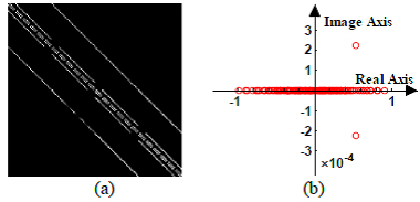
Figure 3: The characteristics of
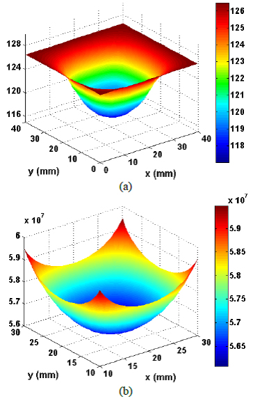
Figure 4: Temperature-dependent parameters of the resistor. (a) . (b) K.
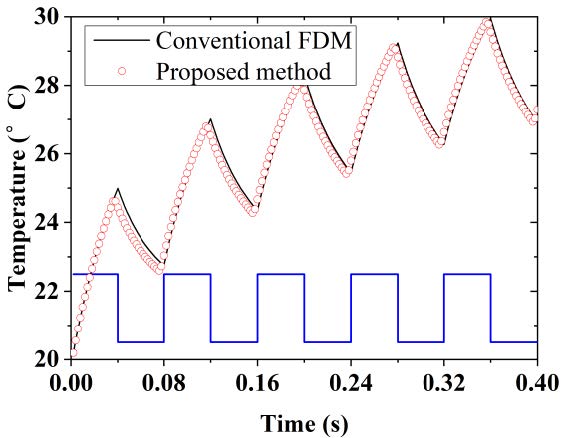
Figure 5: Comparison of the temperatures obtained with the different methods at (20, 20, and 20 mm).

Figure 6: Temperature distribution on the top surface.
Figure 3(a) shows the element distribution characteristics of
The resistor’s and on the top surface at t = 5 s is simulated and given in Figure 4(a) and (b), respectively. Obviously, they are spatially distributed, which is caused by the temperature change in space.
The transient temperatures at (20, 20, and 20 mm) are observed and illustrated in Figure 5. These results are compared with those of the conventional FDM, which adopts a uniform fine grid with mm and its time step is 0.001 s. From the figure, we can see that their numerical results agree well.
Figure 6 shows the temperature distributions on the top surface of the substrate at t = 5 s. We can clearly see that on the boundary of the coarse and fine grids, the temperatures of the coarse grids naturally transit to the fine grids.
In order to further verify the efficiency of the proposed algorithm, the temperatures on the top surface, whose grid numbers are 1576–1800, are also compared with the results from COMSOL software ( s). Figure 7 shows the numerical results of the three methods. Obviously, they are in good agreement. It verifies the effectiveness of the proposed subgridding approach in modeling the multiscale electro-thermal structure.
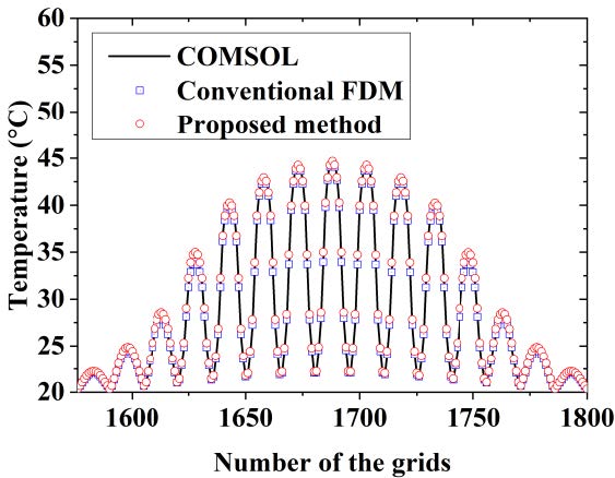
Figure 7: Temperature distribution obtained by COMSOL, conventional method, and the proposed method.
Table 2 lists the computational expenditures of three methods. Based on the table, the following observations are made.
• The proposed algorithm with subgrids reduces the number of unknowns by about 91% and the computational time by about 49.6% compared to the traditional FDM with uniform fine mesh.
• The proposed finite difference subgridding method reduces the number of unknowns by about 70% and the computational time by about 10.7% compared to the COMSOL software.
Table 2: Computational expenditures of different methods
| 31,752 | 5000 | 21.27 | |
| 9391 | N/A | 12.00 | |
| 2825 | 1250 | 10.72 |
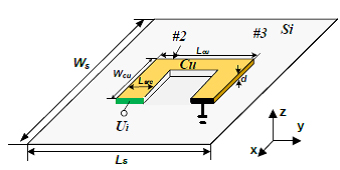
Figure 8: N-shaped resistor integrated on a Si substrate.
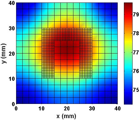
Figure 9: Temperature distribution of the substrate at t = 20 s.
B. N-shaped resistor integrated on a Si substrate
To further study the adaptability of the proposed algorithm, an n-shaped copper resistor (L= W= 20 mm, L= 5 mm, d = 0.1 mm) integrated on a square silicon film substrate (L= W= 40 mm) is illustrated as Figure 9 shows. This model has a multiscale structure. In this case, the square wave voltage changes to be 5 V and its period is 1 s. Other parameters are the same as the square resistance above.
Figure 9 shows the temperature distributions of the substrate at t = 20 s. Also, the obvious reflection of the temperature field on the boundary was not observed. These results are compared with those of the conventional FDM, which adopts a uniform fine grid with mm and its time step is 0.001 s. Figure 10 gives the comparison of the transient temperatures obtained with the two different methods at the observed point (20 and 20 mm). From the figure, we can see that the three temperature patterns tend to be in good agreement. It verifies the effectiveness of the proposed subgridding approach again.
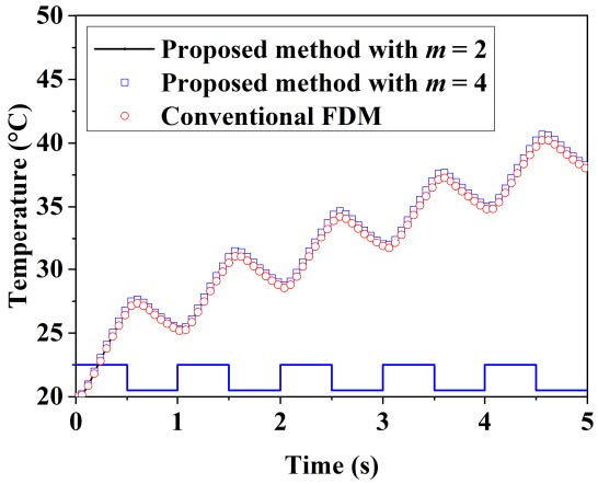
Figure 10: Comparison of the temperatures obtained with the different methods at (20 and 20 mm).
IV. CONCLUSION
In this paper, a 3D explicit finite difference subgridding method is proposed and applied to study the electro-thermal problems of electronic components and ICs with multiscale structures. Square- and n-shaped resistances are used as examples. In order to agree with the actual problems, the temperature-dependent electrical conductivity and thermal conductivity are considered in this research. In addition, the Robbin boundary condition is used in the model. Therefore, the coefficient matrix of the subgridding algorithm is asymmetric. Fortunately, its main diagonal elements are dominant and symmetric; the imaginary part of the other asymmetric elements is close to 0. Based on these properties, the stability condition of the algorithm is derived by matrix method. The numerical results are compared with those of the traditional FDM with fine mesh and the COMSOL software as well. They are in good agreement. In addition, the proposed method can reduce the number of unknowns by about 91% and 70% and the computational time by about 49.6% and 10.7%, compared to the traditional FDM and the COMSOL software, respectively. All of the above show the efficiency of the proposed method.
ACKNOWLEDGMENT
The authors wish to acknowledge the support of the National Natural Science Foundation of China under Grant 61761017.
REFERENCES
[1] J. Xie and M. Swaminathan, “Electrical-thermal Co-simulation of 3D integrated systems with micro-fluidic cooling and Joule heating effects,” IEEE Transactions on Components, Packaging, and Manufacturing Technology, vol. 1, no. 2, pp. 234-246, Feb. 2011.
[2] X. Guan, X. Wei, X. Song, N. Shu, and H. Peng, “FE analysis on temperature, electromagnetic force and load capacities of imperfect assembled GIB plug-in connectors,” Applied Computational Electromagnetics Society Journal, vol. 33, no. 6, pp. 697-705, Jun. 2018.
[3] S. Yanagawa, “Analytical approach to evaluate thermal reduction effects of peripheral structures on microwave power GaAs device chips,” IEEE Microwave and Wireless Components Letters, vol. 15, no. 5, pp. 324-326, May 2005.
[4] B. Vermeersch and G. De Mey, “Dynamic electrothermal simulation of integrated resistors at device level,” Microelectronics Journal, vol. 40, no. 9, pp. 1411-1416, Dec. 2008.
[5] X. Zhang, Z. Chen, and Y. Yu, “An unconditional stable meshless ADI-RPIM for simulation of coupled transient electrothermal problems,” IEEE Journal on Multiscale and Multiphysics Computational Techniques, vol. 1, pp. 98-106,Nov. 2016.
[6] D. I. Doukas, T. A. Papadopoulos, A. I. Chrysochos, D. P. Labridis, and G. K. Papagiannis, “Multiphysics modeling for transient analysis of Gas-insulated lines,” IEEE Transactions on Power Delivery, vol. 33, no. 6, pp. 2786-2793,Dec. 2018.
[7] J. Chai, G. Dong, and Y. Yang, “Nonlinear electrothermal model for investigating transient temperature responses of a through-silicon via array applied with Gaussian pulses in 3-D IC,” IEEE Transactions on Electron Devices, vol. 66, no. 2, pp. 1032-1040, Feb. 2019.
[8] H. Cao, P. Ning, X. Wen, T. Yuan, and H. Li, “An electro-thermal model for IGBT based on finite differential method,” IEEE Journal of Emerging and Selected Topics in Power Electronics, vol. 8, no. 1, pp. 673-684, Mar. 2020.
[9] A. M. Milovanovic, B. M. Koprivica, A. S. Peulic, and I. L. Milankovic, “Analysis of square coaxial line family,” Applied Computational Electromagnetics Society Journal, vol. 30, no. 1, pp. 99-108, Jan. 2015.
[10] M. Moradi, R. S. Shirazi, and A. Abdipour, “Design and non-linear modeling of a wide tuning range four-plate MEMS varactor with high Q-factor for RF application,” Applied Computational Electromagnetics Society Journal, vol. 31, no. 2, pp. 180-186, Feb. 2016.
[11] J. Chen, S. Yang, and Z. Ren, “A network topological approach-based transient 3-D electrothermal model of insulated-gate Bipolar transistor,” IEEE Transactions on Magnetics, vol. 56, no. 2, pp. 1-4, Feb. 2020.
[12] F. Kaburcuk and A. Z. Elsherbeni, “Temperature rise and SAR distribution at wide range of frequencies in a human head due to an antenna radiation,” Applied Computational Electromagnetics Society Journal, vol. 33, no. 4, pp. 367-372, Apr. 2018.
[13] S. S. Zivanovic, K. S. Yee and K. K. Mei, “A subgridding method for the time-domain finite-difference method to solve Maxwell’s equations,” IEEE Transactions on Microwave Theory and Techniques, vol. 39, no. 3, pp. 471-479,Mar. 1991.
[14] K. Xiao, D. J. Pommerenke and J. L. Drewniak, “A three-dimensional FDTD subgridding algorithm with separated temporal and spatial interfaces and related stability analysis,” IEEE Transactions on Antennas and Propagation, vol. 55, no. 7, pp. 1981-1990, Jul. 2007.
[15] J. Chen, A. Zhang, “A subgridding scheme based on the FDTD method and HIE-FDTD method,” Applied Computational Electromagnetics Society journal, vol. 26, no. 1, pp. 1-7,Jan. 2011.
[16] H. AL-Tameemi, J. Bérenger, and F. Costen, “Singularity problem with the one-sheet huygens subgridding method,” IEEE Transactions on Electromagnetic Compatibility, vol. 59, no. 3, pp. 992-995, Jun. 2017.
[17] K. Zeng, and D. Jiao, “Symmetric positive semi-definite FDTD subgridding algorithms in both space and time for accurate analysis of inhomogeneous problems,” IEEE Transactions on Antennas and Propagation, vol. 68, no. 4, pp. 3047-3059, Jan. 2020.
[18] S. Wang, “Numerical examinations of the stability of FDTD subgridding schemes,” Applied Computational Electromagnetics Society Journal, vol. 22, no. 2, pp. 189-194, Jul. 2007.
BIOGRAPHIES

Xianyan Zhang received the B.S. degree in applied physics and the M.S. degree in physical electronics from Yunnan University, Kunming, China, in 2001 and 2004, respectively, and the Ph.D. degree in electromagnetic field and microwave technology from the Institute of Electronics, Chinese Academy of Sciences, Beijing, China, in 2007.
Her research interests include electromagnetic computation, antenna design and wireless power transmission structure design.

Ruilong Chen was born in Hengyang, Hunan, China, in 1996. He received the B.S. degree in communication engineering from Beijing Union University, Beijing, China, in 2018, and the M.S. degree in communication engineering from East China Jiaotong University, Nanchang, China, in 2021.
He is currently working with Wuxi Leihua Science and Technology Co., Ltd. His research interests focus on electromagnetic computation and radar signal processing.

Aiyun Zhan was born in Nantong, Jiangsu, China, in 1973. She received the B.S. degree from Southwest Jiaotong University, Chengdu, China, in 1997, and he M.S. degree from East China Jiaotong University, Nanchang, China, in 2008. She is currently working with the School of Information Engineering, East China Jiaotong University. Her research interests focus on channel coding and optical communication.
ACES JOURNAL, Vol. 37, No. 2, 168–175.
doi: 10.13052/2022.ACES.J.370204
© 2021 River Publishers