A Memory-Efficient Hybrid Implicit–Explicit FDTD Method for Electromagnetic Simulation
Faxiang Chen and Kang Li
1School of Information Science and Engineering, Shandong University, Qingdao 266237, China
cfxlongman@163.com, kangli@sdu.edu.cn
Submitted On: August 15, 2021; Accepted On: February 8, 2022
Abstract
As the explicit finite-difference time-domain (FDTD) method is restricted by the CourantFriedrichLevy (CFL) stability condition and inefficient for simulation in some situations, implicit methods are developed. The hybrid implicitexplicit (HIE) FDTD method is one popular method among them. In this paper, a memory-efficient HIE FDTD method is designed for electromagnetic simulation. The proposed HIE-FDTD method is based upon the divergence relationship of electric fields, nearly reduces one field component, and realizes a memory reduction rate of 33% approximately. Two numerical experiments are carried out to validate the proposed method and the results indicate that the proposed memory-efficient HIE-FDTD method can work well.
Keywords: Finite-difference time-domain (FDTD), hybrid implicitexplicit FDTD (HIE-FDTD), memory-efficient.
I. INTRODUCTION
Solving electromagnetic (EM) field is a necessary part in device design and analysis of EM phenomena, and many methods such as ray tracing method [1], scatter matrix method (SMM) [2–4], and WentzelKramersBrillouin (WKB) method [5] have been proposed. Methods with analytical approximation are relatively accurate and full of physical information, while their scopes are limited. As a result, numerical methods are also developed. The finite-difference time-domain (FDTD) method [6] has been regarded as one of the most effective and versatile methodologies [7, 8] mainly due to its direct temporal computing and simplicity. However, the explicit FDTD method is constrained by the CourantFriedrichLevy (CFL) stability condition [9]. As a result, when there are fine structures in the computation task, the FDTD method has to employ relatively small cell sizes and, thus, unavoidably takes a relatively small time step and consequently is confronted with heavy burden of long running time. In order to solve the issue, researchers resort to implicit schemes and have proposed a series of methods such asalternating-direction implicit (ADI) FDTD method [10, 11], locally one-dimensional (LOD) FDTD method [12, 13], CrankNicolson (CN) FDTD method [14, 15], weighted Laguerre polynomial (WLP) FDTD method [16, 17], and hybrid implicitexplicit (HIE) FDTD method [18, 19]. Among those methods, the ADI-FDTD method and the LOD-FDTD method both employ time split schemes and seem somewhat complex. The CN-FDTD method and the WLP-FDTD method both adopt fully implicit schemes and result in a huge sparse matrix which is expensive to handle. Whereas, the HIE-FDTD method only executes implicit difference schemes for the spatial partial derivatives in the direction along which there are fine structures and takes general explicit difference schemes for the remaining spatial partial derivatives in the directions along which there are no fine elements. In such an arrangement, the HIE-FDTD method finishes the restriction of the fine spatial cell sizes on time step size, acquires the ability to improve computational efficiency, and has drawn much attention in recent years [19–22]. Compared with the conventional FDTD method and even some other absolutely stable FDTD methods such as the ADI-FDTD method in some situations [23], the HIE-FDTD method showed higher efficiency, and a lot of work including but not limited to simulations of designing devices, implementations of PML, and reducing numerical dispersion error [19–22, 24] have been put forward.
Compared with the FDTD method, the HIE-FDTD method becomes more complex and needs more memory to implement, and, recently, the authors in [25] also point out that the character exists in some previous algorithms that employ implicit schemes. As a result, a form of HIE-FDTD method that is both free of strict CFL stability condition and is also of low memory requirements without bringing much complexity may be of value. In the paper [26], the authors proposed a scheme based on divergence relationship and achieved a memory reduction rate near to 33%. Then the thought of memory saving was adopted into some other situations [27–29] in different ways.
In this paper, based on the work proposed in [18] and [26], a memory-efficient HIE-FDTD method is developed based on the divergence relationship of electric fields. It will be seen that the proposed HIE-FDTD method nearly only stores two field components in computation, reduces 33.33% of memory approximately, and maintains the accuracy and efficiency of the original method.
II. ALGORITHM FORMULATION
In simple, isotropic, and lossless media, according to [18], the HIE FDTD method is
| (1) |
| (2) |
| (3) |
In order to acquire the solutions, a user either replaces in eqn (1) with in eqn (3), solves matrix equations, and acquires or inserts eqn (1) into eqn (3), handles matrix equations, and solves and, in the end, calculates the remaining field variables explicitly. We term them as HIE-E-FDTD method and HIE-H-FDTD method, respectively.
The divergence relationship of electric fields can be directly written as
| (4) | |
Eqn (4) can also be rewritten as
| (5) | |
Clearly, the divergence relationship is time invariant. The initial condition is 0; so eqn (5) can be further rewritten as
| (6) |
In fact, eqn (6) is just the result of linear combination of the two curl equations of electric field components in the HIE-FDTD method. In the region containing source, eqn (6) may fail; so one can directly apply the HIE-FDTD method without any change and construct linear equations to solve the fields or get the discrete divergence relationship by directly adding the numerical expressions of the two field components in the conventional HIE-FDTD method according to the regular form of divergence relationship.
Conductor (PEC) will also destroy eqn (6). On the surface of conductor, tangential is 0; so eqn (6) is omitted. As to normal , we recommend using the HIE-FDTD method on surface of conductor directly.
After applying finite difference approximation to spatial derivatives, the full numerical form of eqn (6) can be written as
| (7) |
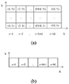
In the computation domain, cells with the same x coordinate are defined as a sub-region registered as x = i. In this paper, each sub-region is rectangle, and the domain consists of cells and is grouped into many rectangles like x = i 1, x = i, and x = i + 1, which is shown in Figure 1.
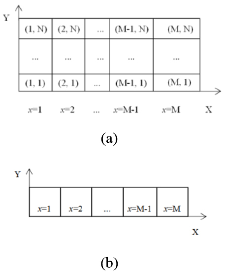
Figure 1: (a) The computation domain with cells and sub-regions. (b) The computation domain with sub-regions.
Fields in these regions are expressed as vectors and registered as , , and . From eqn (7), it can be seen that in x = i only requires in x = i 1 except in x = i and in x = i and in x = i 1. In this paper, fields are at sides of cells in y direction, fields are at sides of grids in x direction, and fields are at the centers of each cell. As a result, eqn (7) can also be rewritten as a matrix form
| (8) |
where , and are matrices determined by coefficients in front of fields in eqn (7).
Suppose x = i 1 is the initial position where our calculation begins. We define and where k can be each rectangle in the whole domain. As to , only two vectors that can store in x = i 1 and that has the memory sufficient to store in x = i are defined.
First, as is equal to in x = i 1, can be valued through eqn (8) and is equal to in x = i. As , , and are known in x = i 1, and can be solved by the conventional HIE-FDTD procedure in x = i 1. Then = which is equal to in x = i, and in x = i + 1 can be valued by eqn (8) and can reuse the memory occupied by . And now as , and are known in x = i, and and can be solved by the conventional HIE-FDTD procedure in x = i again. Repeating this process to the last rectangle, it will be seen that all and have been solved, and only two vectors that store in each sub-region temporarily and are alternatively used are sufficient to finish the calculation, while in the conventional HIE-FDTD method, all field components are required to store. As a result, in the proposed method, one electric field component is nearly eliminated and the aim of memory reduction is realized in such a way.
A short pseudo-code is written below. Some terms in this content will be explained. In this part, is the last time step, each value of x presents the rectangle corresponding to cells with the same coordinate of x in the computation domain, and presents the last rectangle. and are both vectors, and and are matrices. t presents the current time step in iteration.
Pseudo-code of the proposed method:
Vector stores (=0); = 0; = 0.
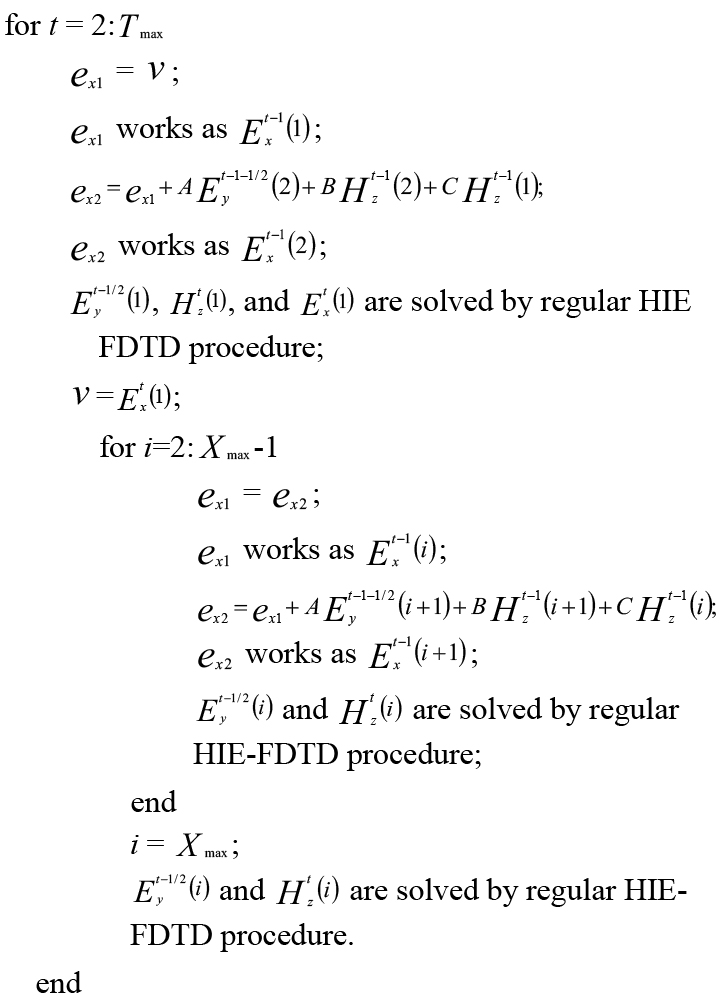
It must be pointed out that and it with identifications of different time steps and space positions both in the description above and in the proposed method only indicate electric fields of x component and does not mean a matrix that is defined, occupies memory and stores fields covering the whole calculation domain.
From the description above, it can be stated that in an arbitrary iteration at (n + 1)th time step, the proposed method does not need to store all the fields beforehand; only two vectors and that are repeatedly used are sufficient for the run of the algorithm, and, in such a way, the memory reduction is realized. In this description, are chosen as unknown variables in linear equations. For the case that works as unknown variables, the algorithm is implemented in a similar way.
In fact, in the proposed method, at each time step, appear in each sub-region by eqn (7) but do not need to store after fields in this region are solved. Supposing in some regions are required, one only needs to store those solutions when the run goes through the local regions.
III. NUMERICAL VALIDATION
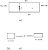
In order to validate the proposed method, two numerical experiments that both use 2D parallel plate waveguides [15] are carried out. The structures used in the two examples are shown in Figure 2.
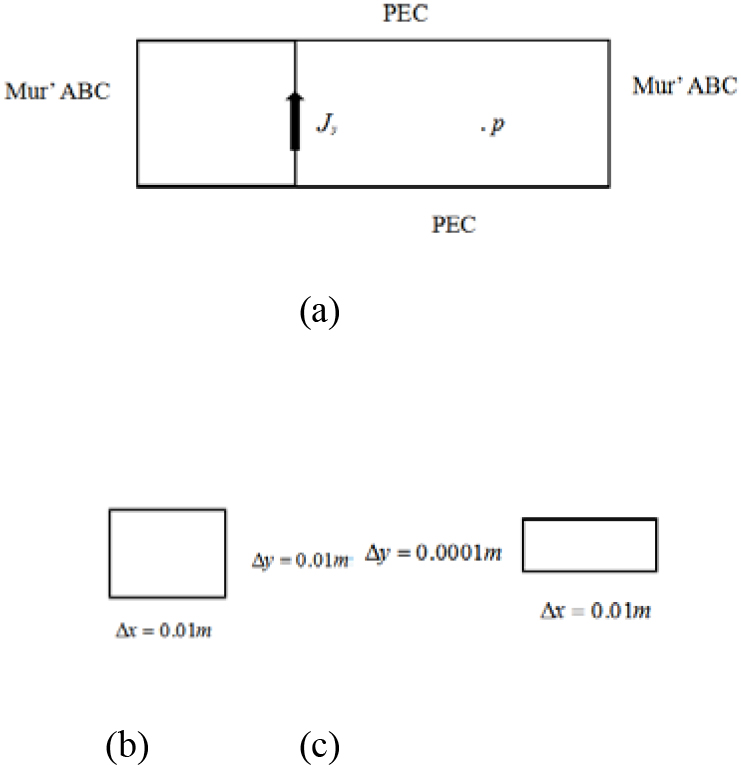
Figure 2: (a) The structures in the two numerical examples, (b) one cell in the first example, and (c) one cell in the second example.
The excitation for the two numerical tests taken from [11] is
| (9) |
where
| (10) | |
In the structure, p is the probe point recording fields at different time step, and is the excitation current.
In the first example, there are 200 and 100 cells with the sizes set as = 0.01 m and = 0.01 m along x and y directions, respectively. The source is placed on line of x = 10 and the point p(50,5) is chosen as observation point recording at each time step and the two sides of the extended waveguide are both truncated by first-order Mur’ absorbing boundary condition. In this situation, according to the CFL stability condition, the largest time step sizes for the conventional FDTD method and the HIE-FDTD method are 23.57 and 33.33 ps, respectively. For the convenience of comparative analysis, the time steps for conventional FDTD and HIE-FDTD methods in this case are both simply set as 20 ps.
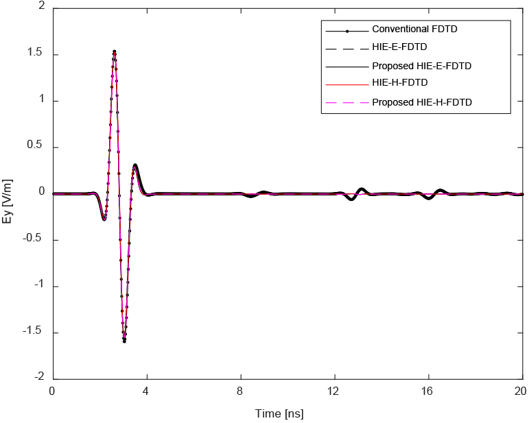
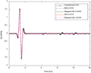
Figure 3: Transient at p point.
Table 1: Comparison of computation time of different methods with uniform time step size
| FDTD methods | Time step | Iteration numbers | CPU time (s) |
|---|---|---|---|
| Conventional FDTD | 20 ps | 1000 | 1.23 |
| Original HIE-E-FDTD | 20 ps | 1000 | 33.35 |
| Proposed HIE-E-FDTD | 20 ps | 1000 | 33.76 |
| Original HIE-H-FDTD | 20 ps | 1000 | 35.58 |
| Proposed HIE-H-FDTD | 20 ps | 1000 | 35.71 |
Figure 3 shows at p point and Table 1 records the running time consumed by the FDTD method, HIE-FDTD method, and the proposed memory-efficient version of the later method with the uniform time step size. From Figure 3, we can see that the numerical results supplied by several algorithms are all in good agreement and, thus, validate the correctness of the new memory-efficient version of HIE-FDTD method. It can be seen that different implementations of the HIE-FDTD methods show a little difference in computation time. As the HIE-FDTD method is an implicit method, it costs more time than the conventional FDTD method when a uniform time step is used.
In order to measure the accuracy of the proposed method, is defined as error function. In this function, stands for the total number of time step iterations and equals 1000. The solutions of the original HIE-E-FDTD method and original HIE-H-FDTD method are set as reference solutions when the errors of two implementations of the proposed memory-efficient method are discussed. Setting the solution from the original HIE-E-FDTD method as standard, the error between the original HIE-E-FDTD method and the proposed HIE-E-FDTD method is 0. Setting the solution from the original HIE-H-FDTD method as standard, the error between the original HIE-H-FDTD method and the proposed original HIE-H-FDTD method is 3.59 10. It can be seen that the errors are very small and show almost no difference. So the accuracy of the proposed method can be seen as the same as that of the original HIE-FDTD method.
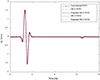
In the second numerical example, we still employ the extended plate waveguide as test model mentioned above but fine the mesh size along y direction to 0.0001 m, and all the other conditions stay the same. The relevant results and time cost are shown in Figure 4 and Table 2.
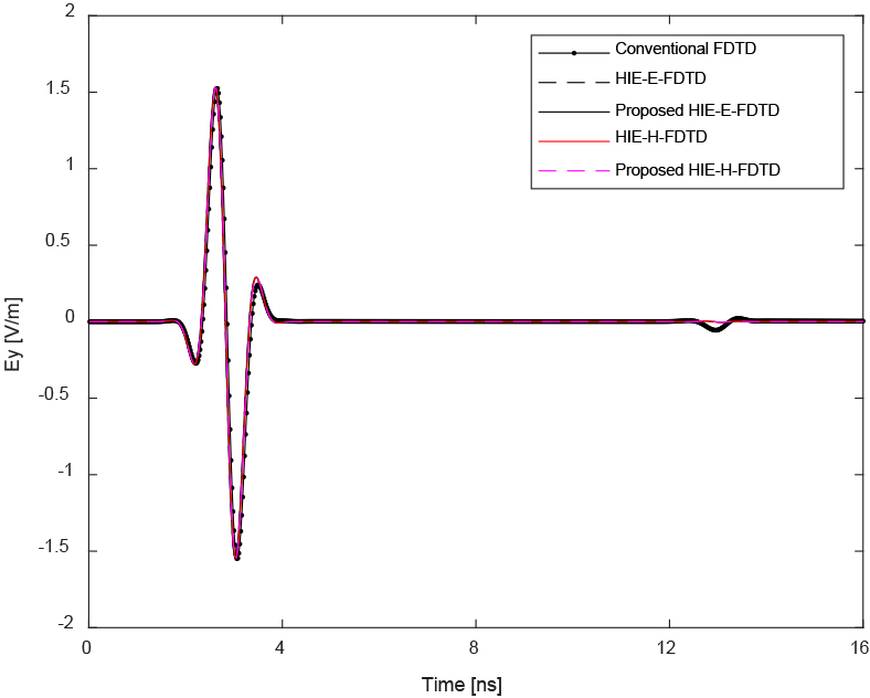
Figure 4: Transient at p point.
Figure 4 still shows that the results calculated by the conventional FDTD method, HIE-FDTD method, and the proposed memory-efficient HIE-FDTD method are all in good agreement.
Table 2 represents the CPU time for the simulations run by different methods. In this situation, it can be seen that different implementations of the HIE-FDTD methods show a little difference in computation time. The proposed method takes almost the same time as the original HIE-FDTD method, while it is still much faster than the conventional FDTD method. As a result, the proposed memory-efficient HIE-FDTD method can both work well for problems with or without fine structures in one direction.
Table 2: Comparison of computation time of different methods with nonuniform time step sizes
| FDTD methods | Time step | Iteration numbers | CPU time (s) |
|---|---|---|---|
| Conventional FDTD | 0.2 ps | 80,000 | 69.60 |
| Original HIE-E-FDTD | 20 ps | 800 | 32.85 |
| Proposed HIE-E-FDTD | 20 ps | 800 | 32.82 |
| Original HIE-H-FDTD | 20 ps | 800 | 29.75 |
| Proposed HIE-H-FDTD | 20 ps | 800 | 29.65 |
Using the same method of measuring the accuracy of the proposed method adopted in the first example, and setting the solution from the original HIE-E-FDTD method as standard, the error between the original HIE-E-FDTD method and the proposed HIE-E-FDTD method is 0. Setting the solution from the original HIE-H-FDTD method as standard, the error between the original HIE-H-FDTD method and the proposed HIE-H-FDTD method is 6.9910. In this function, stands for the total number of time step iterations and equals 800. It can be seen that the errors both are very small and show almost no difference. So the accuracy of the proposed method is the same as that of the original HIE-FDTD method.
Table 3: Memory cost (KB) in different methods
| FDTD (KB) | HIE-E-FDTD |
HIE-H-FDTD | Proposed HIE-E-FDTD | Proposed HIE-H-FDTD | |
|---|---|---|---|---|---|
| A | 468.75 | 468.75 |
468.75 |
314.06 |
314.06 |
| B | 468.75 | 468.75 | 468.75 |
314.06 |
314.06 |
Table 3 shows the memory cost in different methods. As the numbers of cells in two numerical examples are equal, the memory of storing fields they require is also equal and listed in Table 3 where A presents the first numerical example and B presents the second one. It is clear that 1312.50/468,075 33%; so the memory reduction rate is near to 33%.
IV. CONCLUSION
The analytic and semi-analytical methods are accurate and can also show physical aspects of a system explicitly. At the same time, numerical methods are also developed and are available in a wider range. Numerical methods require more memory than analytic methods in most situations. The HIE-FDTD method shows higher computation efficiency than the FDTD method in problems with fine elements in one direction. In this paper, efforts are made to reduce memory cost and a memory-efficient HIE FDTD method is proposed based on divergence relationship of electric fields. The proposed algorithm nearly eliminates one electric field component, saves nearly 33% of memory, and the implementation of the proposed method is not much more complex than the conventional HIE-FDTD method. Numerical experiments are carried out and validate that the proposed memory-efficient HIE-FDTD method can solve EM fields correctly and runs almost as fast as the original HIE-FDTD method, and in those situations, the computational efficiency can be interpreted as unchanged. The accuracy of the proposed memory-efficient HIE-FDTD method is also very close to that of the original HIE-FDTD method.
REFERENCES
[1] L. J. Guo, L. X. Guo, and L. P. Gan, “Influence of dusty plasma on antenna radiation,” Physics of Plasmas, vol. 28, no. 8, p. 083701, Aug. 2021.
[2] L. X. Guo and L. J. Guo, “The effect of the inhomogeneous collision frequency on the absorption of electromagnetic waves in a magnetized plasma,” Physics of Plasmas, vol. 24, no. 11, p. 112119, Nov. 2017.
[3] Q. W. Rao, G. J. Xu, P. F. Wang, and Z. Q. Zheng, “Study on the propagation characteristics of terahertz waves in dusty plasma with a ceramic substrate by the scattering matrix method,” Sensors, vol. 21, no. 263, pp. 1-11, Jan. 2021.
[4] Q. W. Rao, G. J. Xu, P. F. Wang, and Z. Q. Zheng, “Study on the propagation characteristics of terahertz waves in dusty plasma with a ceramic substrate by the scattering matrix method,” International Journal of Antennas and Propagation, vol. 2021, no. 6625530, pp. 1-9, Jan. 2021.
[5] Y. Y. Chen, H. B. Wang, and D. L. Zhao, “The applicability of WKB method in studying inhomogeneous dusty plasma,” IEEE Transactions on Plasma Science, vol. 48, no. 1, pp. 275-279, Jan. 2020.
[6] K. Yee, “Numerical solution of initial boundary value problems involving Maxwell’s equations in isotropic media”, IEEE Trans. Antennas Propag., vol. AP-14, no. 3, pp. 302-307, May1966.
[7] A. Taflove and S. C. Hagness, “Computational electrodynamics: the finite-difference time-domain method,” Norwood, MA, USA: Artech House, 2005.
[8] D. M. Sullivan, Electromagnetic Simulation Using the FDTD Method, Hoboken, NJ, USA:Wiley, 2013.
[9] F. L. Teixeira, “A summary review on 25 years of progress and future challenges in FDTD and FETD techniques,” Applied Computational Electromagnetics Society (ACES) Journal, vol. 25, no. 1, pp. 1-14, Jan. 2010.
[10] T. Namiki, “A new FDTD algorithm based on alternating-direction implicit method”, IEEE Trans. Microw. Theory Techn., vol. 47, no. 10, pp. 2003-2007, Oct. 1999.
[11] J. Chen, “New alternating direction implicit finite-difference time-domain method with higher efficiency,” Applied Computational Electromagnetics Society (ACES) Journal, vol. 27, no. 11, pp. 903-907, Nov. 2012.
[12] T. L. Liang, W. Shao, and S. B. Shi, “Complex-envelope ADE-LOD-FDTD for band gap analysis of plasma photonic crystals,” Applied Computational Electromagnetics Society (ACES) Journal, vol. 33, no. 4, pp. 443-449, Apr.2018.
[13] A. K. Saxena and K. V. Srivastava, “Three-dimensional unconditionally stable LOD-FDTD methods with low numerical dispersion in the desired directions,” IEEE Transactions on Antennas and Propagation, vol. 64, no. 7, pp. 3055-3067, Jul. 2016.
[14] G. L. Sun and C. W. Trueman, “Unconditionally stable Crank–Nicolson scheme for solving two-dimensional Maxwell’s equations”, Electron. Lett., vol. 39, no. 7, pp. 595-597, Apr.2003.
[15] J. X. Li, H. L. Jiang, and N. X. Feng, “Efficient FDTD implementation of the ADE-based CN-PML for the two dimensional TMz waves,” Applied Computational Electromagnetics Society (ACES) Journal, vol. 30, no. 6, pp. 688-691, Jun.2015.
[16] Y. S. Chung, T. K. Sarkar, B. H. Jung, and M. Salazar-Palma, “An unconditionally stable scheme for the finite-difference time-domain method”, IEEE Trans. Microw. Theory Techn., vol. 51, no. 3, pp. 697-704, Mar. 2003.
[17] W. Shao and J. L. Li , “An efficient laguerre-FDTD algorithm for exact parameter extraction of lossy transmission lines,” Applied Computational Electromagnetics Society (ACES) Journal, vol. 27, no. 3, pp. 223-228, Mar.2012.
[18] B. Huang, G. Wang, Y. Jiang, and W. Wang, “A hybrid implicit-explicit FDTD scheme with weakly conditional stability”, Microw. Opt. Technol. Lett., vol. 39, no. 2, pp. 97-101, Oct. 2003.
[19] L. J. Y. Guo, J. Chen, J. G. Wang, and A. X. Zhan, “A new HIE-PSTD method for solving problems with fine and electrically large structures simultaneously,” Applied Computational Electromagnetics Society (ACES) Journal, vol. 31, no. 12, pp. 1397-1340, Dec. 2016.
[20] F. Moharrami and Z. Atlasbaf, “Simulation of multilayer graphene–dielectric metamaterial by implementing SBC model of graphene in the HIE-FDTD method,” IEEE Transactions on Antennas and Propagation, vol. 68, no. 3, pp. 2238-2245, Mar. 2020.
[21] J. Chen, “A review of hybrid implicit explicit finite difference time domain method,” J. Computat. Phys., vol. 363, pp. 256-267, Jun. 2018.
[22] Y. Kong, C. Zhang, and Q. Chu, “An optimized one-step leapfrog HIE-FDTD method with the artificial anisotropy parameters,” IEEE Transactions on Antennas and Propagation, vol. 68, no. 2, pp. 1198-1203, Feb. 2020.
[23] J. Chen and J. Wang, “Comparison between HIE-FDTD method and ADI-FDTD method,” Microw. Opti. Technol. Lett., vol. 49, no. 5, pp. 1001–1005, Mar. 2007.
[24] P. Wu, Y. Xie, H. Jiang, H. Di, and T. Natsuki, “Complex envelope hybrid implicit-explicit procedure with enhanced absorption for bandpass nonreciprocal application,” IEEE Microwave and Wireless Components Letters, vol. 31, no. 6, pp. 533-536, Jun. 2021.
[25] K. L. Zhang, L. Wang, R. P. Li, M. J. Wang, C. Fan, H. X. Zheng, and E. P. Li., “Low-dispersion leapfrog WCS-FDTD with artificial anisotropy parameters and simulation of hollow dielectric resonator antenna array,” IEEE Transactions on Antennas and Propagation. vol. 69, no, 9, pp. 5810-5811, Sep. 2021.
[26] G. D. Kondylis, F. De Flaviis, G. J. Pottie, and T. Itoh, “A memory-efficient formulation of the finite-difference time-domain method for the solution of Maxwell equations,” IEEE Transactions on Microwave Theory and Techniques, vol. 49, no. 7, pp. 1310-1320, Jul. 2001.
[27] Y. Yi, B. Chen, W. Sheng, and Y. Pei, “A memory-efficient formulation of the unconditionally stable FDTD method for solving Maxwell’s equations,” IEEE Transactions on Antennas and Propagation, vol. 55, no. 12, pp. 3729-3733, Dec. 2007.
[28] B. Liu, B. Q. Gao, W. Tan, and W. Ren, “A new FDTD algorithm - ADI/R-FDTD”, Electromagnetic Compatibility 2002 3rd International Symposium, pp. 250-253, May 2002.
[29] T. B. Yu and B. H Zhou, “A memory-efficient FDTD algorithm for solving Maxwell equations in cylindrical grids,” IEEE Transactions on Antennas and Propagation, vol. 52, no. 5, pp. 1382-1384, May 2004.
BIOGRAPHIES

Kang Li was born in Jinan, China, in 1962. He received the B.S. and M.S. degrees in electrical engineering and the Ph.D. degree in optical engineering from Shandong University, Jinan, China, in 1984, 1987, and 2006, respectively.
He is currently a Professor with the School of Information Science and Engineering, Shandong University. His current research interests include computational electromagnetics and fiber-optic communications.

Faxiang Chen received the master’s degree in electromagnetic field and microwave technology from Shanghai Maritime University, Shanghai, China, in 2015. He is currently working toward the Ph.D. degree in electronic science and technology with the Shandong University, Qingdao, China.
His current research interest includes computational electromagnetics.
ACES JOURNAL, Vol. 37, No. 2, 149–155.
doi: 10.13052/2022.ACES.J.370202
© 2021 River Publishers