Formulation of Iterative Finite-Difference Method for Generating Large Spatially Variant Lattices

Manuel F. Martinez${}^{\mathbf{\text{1}}}$, Jesus J. Gutierrez${}^{\mathbf{\text{1}}}$, Jimmy E. Touma${}^{\mathbf{\text{2}}}$, and Raymond C. Rumpf${}^{\mathbf{\text{1}}}$

¹Department of Electrical and Computer Engineering, University of Texas at El Paso, El Paso, TX 79968, USA
mfmartinez4@miners.utep.edu, jjgutierrez4@utep.edu, rcrumpf@utep.edu

²Air Force Research Laboratory, Integrated Sensing and Processing, Eglin Air Force Base, Eglin, FL 32542, USA
jimmy.touma.1@us.af.mil

Submitted On: August 31, 2021; Accepted On: February 8, 2022

Abstract

A new numerical method to generate spatially variant lattices (SVLs) is derived and implemented. The algorithm proposed solves the underlying partial differential equations iteratively with an update equation derived using the finite-difference method to obtain an SVL that is continuous, smooth, and free of unintended defects while maintaining the unit cell geometry throughout the lattice. This iterative approach is shown to be more memory-efficient when compared to the matrix-based approach and is, thus, suitable for the calculation of large-scale SVLs. The iterative nature of the solver allows it to be easily implemented in graphics processing unit to parallelize the computation of SVLs. Two spatially variant self-collimating photonic crystals are generated and simulated to demonstrate the functionality of the algorithm as a tool to generate fully three-dimensional photonic devices of realistic size.

Keywords: Iterative finite-difference method, functionally graded, metamaterials, photonic crystals, spatial variance.

I. INTRODUCTION

Self-collimating photonic crystals (SCPCs) are devices in which an electromagnetic wave travels through a volume of material without any diffraction and only moves along an axis of the lattice regardless of angle of incidence [1]. Attempts to control power flow inside these structures in an arbitrary manner in 3D SCPCs have been limited to the introduction of defects or deformations [2], which often weaken or destroy the overall electromagnetic properties of the SCPC. Spatial variance is a process to spatially adjust the geometrical aspects of periodic structures like photonic crystals (PhCs) [3]. The algorithm for spatial variance introduces geometrical changes to the PhC in a way that makes the PhC smooth, continuous, and free of unintentional defects [4] while retaining the geometry of the unit cells so that electromagnetic response is maintained. Most approaches to incorporate spatial variance in SCPCs [5–7] do so in either planar SCPCs or with devices in which the third dimension is not spatially varied. The method described in [3] suffers from the major drawback of being memory inefficient due to its reliance on large full storage matrices and computationally expensive lower–upper (LU) decomposition operations, thus limiting the size of spatially variant lattices (SVLs) that can be generated. Although other methods such as Galerkin, Crank-Nicolson, and Fourier methods [8] exist to solve partial differential equations, these run into the similar drawbacks of memory inefficiency when solving large problems. The present body of work discusses the formulation of an iterative algorithm to compute SVLs based on similar approaches to those used in electromagnetic simulation tools such as the finite-difference time-domain (FDTD) method, in which an update equation is used to explicitly solve the underlying system of partial differential equations point-by-point throughout the problem space [9]. Approaches with similar formulations to the one presented in this body of work have been successfully implemented with the use of general purpose graphics processing units (GPGPUs) to accelerate and scaleexecution [10].

II. GENERATION OF SPATIALLY VARIANT LATTICES

In this section, the step-by-step description of the overall algorithm to generate SVLs is presented. The first two subsections discuss the mathematical background of spatially variant gratings and SVLs. The following subsections define the steps necessary to calculate an SVL using the iterative algorithm as well as presenting the flow-diagram of the proposedalgorithm.

A. Spatially variant planar gratings and lattices

Consider a simple sinusoidal grating described by a grating vector $\overrightarrow{K}$. The grating vector has a direction perpendicular to the planes of the grating and has a magnitude of $2\pi /\mathrm{\Lambda }$, where $\mathrm{\Lambda }$ is the period of the grating. Given a grating vector, the sinusoidal grating is calculated by

$${\epsilon }_a(\overrightarrow{s})=\cos (\overrightarrow{K}\bullet \overrightarrow{s}),$$

(1)

where $\overrightarrow{s}=x{\widehat{a}}_x+y{\widehat{a}}_y+x{\widehat{a}}_z$ and ${\epsilon }_a(\overrightarrow{s})$ is called the analog grating because of its continuous variation between the values of $-$1 and 1.

When attributes of the grating such as period or the orientation are spatially varied, the grating vector $\overrightarrow{K}$ becomes a function of position. When this happens, $\overrightarrow{K}$ becomes $\overrightarrow{K}(\overrightarrow{s})$ and the calculation in eqn (1) fails to properly compute the analog grating [3]

$${\epsilon }_a(\overrightarrow{s})\ne \cos \left[\overrightarrow{K}(\overrightarrow{s})\bullet \overrightarrow{s}\right].$$

(2)

Spatial variance is incorporated through an intermediate parameter called the grating phase $\mathrm{\Phi }(\overrightarrow{s})$ [3]. The equation shown in eqn (3) is solved numerically through a best fit approach of least squares since there are more equations than unknowns. Then, the analog grating can be calculated by eqn (4)

$$\nabla \mathrm{\Phi }(\overrightarrow{s})=\overrightarrow{K}(\overrightarrow{s}),$$

(3)

$${\epsilon }_a(\overrightarrow{s})=\cos \left[\mathrm{\Phi }(\overrightarrow{s})\right].$$

(4)

To extend the functionality of eqn (3) and (4) from planar gratings to general lattices, Rumpf [3] states that the unit cell that describes the periodic structure to be spatially varied is decomposed into a complex Fourier series. Each term in the Fourier series is a spatial harmonic that can be interpreted as a one-dimensional planar grating. Given the infinite nature of Fourier transforms, this complex series is truncated to only a finite set of markedasmathitalicM planar gratings. Each planar grating in the truncated series is spatially varied and the overall SVL is obtained by summing each 1D grating.

B. A general solution for $\nabla \mathrm{\Phi }(\overrightarrow{s})=\overrightarrow{K}(\overrightarrow{s})$

Rumpf [3] presented a matrix-based numerical solution for the expression in eqn (3) in the framework of least squares with the use of ${[A]}^{-1}[b]=[x]$. This implementation is a brute force approach that provides fast and accurate results for small-sized problems. The issue with this approach to the solution arises when large-scale lattices are being generated since the ${[A]}^{-1}[b]=[x]$ is a matrix problem that increases memory and computational requirements. This poor scaling with larger lattices leads to a hard-set limit of the size of lattice that can be computationally generated.

III. ITERATIVE SOLUTION TO $\nabla \mathrm{\Phi }(\overrightarrow{s})=\overrightarrow{K}(\overrightarrow{s})$

A. The update equation

The derivation of the fundamental equations to iteratively generate SVLs begins by expanding the expression to be solved in eqn (3) into Cartesian coordinates

$$\frac{\partial \mathrm{\Phi }(\overrightarrow{s})}{\partial x}+\frac{\partial \mathrm{\Phi }(\overrightarrow{s})}{\partial y}+\frac{\partial \mathrm{\Phi }(\overrightarrow{s})}{\partial z}=K_x(\overrightarrow{s}){\widehat{a}}_x+K_y(\overrightarrow{s}){\widehat{a}}_y+K_z(\overrightarrow{s}){\widehat{a}}_z.$$

(5)

This vector equation can be separated into three independent scalar equations by setting the vector components on each side of the equation equal

$$\frac{\partial \mathrm{\Phi }(\overrightarrow{s})}{\partial x}=K_x(\overrightarrow{s}),$$

(6)

$$\frac{\partial \mathrm{\Phi }(\overrightarrow{s})}{\partial y}=K_y(\overrightarrow{s}),$$

(7)

$$\frac{\partial \mathrm{\Phi }(\overrightarrow{s})}{\partial z}=K_z(\overrightarrow{s}).$$

(8)

For brevity, the following formulation focuses on eqn (6) as the basic building block for the update equation and then applied by inspection to the other equations. Eqn (6) can be approximated by a central finite-difference to the $\mathit{\text{i}}-1$ side or a central finite-difference to the $\mathit{\text{i}}+1$ side

$$\frac{{\mathrm{\Phi }|}_{i,j,k}-{\mathrm{\Phi }|}_{i-1,j,k}}{\mathrm{\Delta }x}=\frac{{K_x|}_{i,j,k}+{K_x|}_{i-1,j,k}}{2}i-1.$$

(9)

$$\frac{{\mathrm{\Phi }|}_{i+1,j,k}-{\mathrm{\Phi }|}_{i,j,k}}{\mathrm{\Delta }x}=\frac{{K_x|}_{i+1,j,k}+{K_x|}_{i,j,k}}{2}i+1.$$

(10)

Solving eqn (9) and (10) for ${\mathrm{\Phi }|}_{i,j,k}$ results in

$${\mathrm{\Phi }|}_{i,j,k}=\frac{{\mathrm{\Phi }|}_{i-1,j,k}+{\mathrm{\Phi }|}_{i+1,j,k}}{2}+\frac{\mathrm{\Delta }x}{4}({K_x|}_{i-1,j,k}-{K_x|}_{i+1,j,k}).$$

(11)

In order to generate the grating phase term iteratively, eqn (11) needs to be interpreted as an update equation, where a new term of ${\mathrm{\Phi }|}_{i,j,k}$ is calculated at each iteration based on an old value of ${\mathrm{\Phi }|}_{i,j,k}$ at a previous iteration. Then, eqn (11) is written as

${{\mathrm{\Phi }}_{\mathrm{new}}|}_{i,j,k}={\displaystyle \frac{{{\mathrm{\Phi }}_{\mathrm{old}}|}_{i-1,j,k}+{{\mathrm{\Phi }}_{\mathrm{old}}|}_{i+1,j,k}}{2}}+$
${\displaystyle \frac{\mathrm{\Delta }x}{4}}({K_x|}_{i-1,j,k}-{K_x|}_{i+1,j,k}).$	(12)

Observing eqn (3.1), this problem consists of a system with more equations than unknowns. It is not possible to satisfy this system of equations exactly to obtain ${{\mathrm{\Phi }}_{\mathrm{new}}|}_{i,j,k}$. Instead, a least-squares approach was used to solve this system of equations. To incorporate the least-squares framework into eqn (3.1), three error terms are included in the formulation that should be minimized

${{\mathrm{\Phi }}_{\mathrm{new}}|}_{i,j,k}={\displaystyle \frac{{{\mathrm{\Phi }}_{\mathrm{old}}|}_{i-1,j,k}+{{\mathrm{\Phi }}_{\mathrm{old}}|}_{i+1,j,k}}{2}}+{\displaystyle \frac{\mathrm{\Delta }x}{4}}\left({K_x|}_{i-1,j,k}-{K_x|}_{i+1,j,k}\right)+{\epsilon }_1.$
${{\mathrm{\Phi }}_{\mathrm{new}}|}_{i,j,k}={\displaystyle \frac{{{\mathrm{\Phi }}_{\mathrm{old}}|}_{i,j-1,k}+{{\mathrm{\Phi }}_{\mathrm{old}}|}_{i,j+1,k}}{2}}+{\displaystyle \frac{\mathrm{\Delta }y}{4}}\left({K_y|}_{i,j-1,k}-{K_y|}_{i,j+1,k}\right)+{\epsilon }_2.$
${{\mathrm{\Phi }}_{\mathrm{new}}|}_{i,j,k}={\displaystyle \frac{{{\mathrm{\Phi }}_{\mathrm{old}}|}_{i,j,k-1}+{{\mathrm{\Phi }}_{\mathrm{old}}|}_{i,j,k+1}}{2}}+{\displaystyle \frac{\mathrm{\Delta }z}{4}}\left({K_z|}_{i,j,k-1}-{K_y|}_{i,j,k+1}\right)+{\epsilon }_3.$	(13)

Solving for each error term in eqn (3.1) yields

${\epsilon }_1={{\mathrm{\Phi }}_{\mathrm{new}}|}_{i,j,k}-{\displaystyle \frac{{{\mathrm{\Phi }}_{\mathrm{old}}|}_{i-1,j,k}+{{\mathrm{\Phi }}_{\mathrm{old}}|}_{i+1,j,k}}{2}}-{\displaystyle \frac{\mathrm{\Delta }x}{4}}\left({K_x|}_{i-1,j,k}-{K_x|}_{i+1,j,k}\right).$
${\epsilon }_2={{\mathrm{\Phi }}_{\mathrm{new}}|}_{i,j,k}-{\displaystyle \frac{{{\mathrm{\Phi }}_{\mathrm{old}}|}_{i,j-1,k}+{{\mathrm{\Phi }}_{\mathrm{old}}|}_{i,j+1,k}}{2}}-{\displaystyle \frac{\mathrm{\Delta }x}{4}}\left({K_x|}_{i,j-1,k}-{K_x|}_{i,j+1,k}\right).$
${\epsilon }_3={{\mathrm{\Phi }}_{\mathrm{new}}|}_{i,j,k}-{\displaystyle \frac{{{\mathrm{\Phi }}_{\mathrm{old}}|}_{i,j,k-1}+{{\mathrm{\Phi }}_{\mathrm{old}}|}_{i,j,k+1}}{2}}-{\displaystyle \frac{\mathrm{\Delta }x}{4}}\left({K_x|}_{i,j,k-1}-{K_x|}_{i,j,k+1}\right).$	(14)

In the least-squares framework, the overall error metric markedasmathitalicE to minimize is defined as

$$\mathit{\text{E}}={\epsilon }_1^2+{\epsilon }_2^2+{\epsilon }_3^2.$$

(15)

To minimize the error in eqn (15), the first-derivative rule is used, resulting in

$$0=\frac{d}{{d{\mathrm{\Phi }}_{\mathrm{new}}|}_{i,j,k}}({\epsilon }_1^2+{\epsilon }_2^2+{\epsilon }_3^2).$$

(16)

Incorporating the error term into eqn (3.1)

${{\mathrm{\Phi }}_{\mathrm{new}}|}_{i,j,k}=$
${\displaystyle \frac{1}{3}}\left[{\displaystyle \frac{{{\mathrm{\Phi }}_{\mathrm{old}}|}_{i-1.j,k}+{{\mathrm{\Phi }}_{\mathrm{old}}|}_{i+1,j,k}}{2}}+{\displaystyle \frac{\mathrm{\Delta }x}{4}}\left({K_x|}_{1-1,j,k}-{K_x|}_{1+1,j,k}\right)\right]$
$+{\displaystyle \frac{1}{3}}\left[{\displaystyle \frac{{{\mathrm{\Phi }}_{\mathrm{old}}|}_{i.j,-1,k}+{{\mathrm{\Phi }}_{\mathrm{old}}|}_{i,j+1,k}}{2}}+{\displaystyle \frac{\mathrm{\Delta }x}{4}}\left({K_x|}_{1,j-1,k}-{K_x|}_{1,j+1,k}\right)\right]$
$+{\displaystyle \frac{1}{3}}\left[{\displaystyle \frac{{{\mathrm{\Phi }}_{\mathrm{old}}|}_{i.j,k-1}+{{\mathrm{\Phi }}_{\mathrm{old}}|}_{i,j,k+1}}{2}}+{\displaystyle \frac{\mathrm{\Delta }x}{4}}\left({K_x|}_{1,j,k-1}-{K_x|}_{1,j,k+1}\right)\right].$	(17)

Comparing the terms inside the square brackets in eqn (3.1) to eqn (3.1) shows that solving the system of equations in eqn (3.1) by least squares is the same as calculating the arithmetic mean of the value of ${{\mathrm{\Phi }}_{\mathrm{new}}|}_{i,j,k}$ generated by solving eqn (3.1) individually. Therefore, the calculation for ${{\mathrm{\Phi }}_{\mathrm{new}}|}_{i,j,k}$ can be written as

$${{\mathrm{\Phi }}_{\mathrm{new}}|}_{i,j,k}=\frac{{{\mathrm{\Phi }}_x|}_{i,j,k}+{{\mathrm{\Phi }}_y|}_{i,j,k}+{{\mathrm{\Phi }}_z|}_{i,j,k}}{3}$$

(18)

where

${{\mathrm{\Phi }}_x|}_{i,j,k}={\displaystyle \frac{{{\mathrm{\Phi }}_{\mathrm{old}}|}_{i-1,j,k}+{{\mathrm{\Phi }}_{\mathrm{old}}|}_{i+1,j,k}}{2}}$
$+{\displaystyle \frac{\mathrm{\Delta }x}{4}}({K_x|}_{i-1,j,k}-{K_x|}_{i+1,j,k}).$
${{\mathrm{\Phi }}_y|}_{i,j,k}={\displaystyle \frac{{{\mathrm{\Phi }}_{\mathrm{old}}|}_{i,j-1,k}+{{\mathrm{\Phi }}_{\mathrm{old}}|}_{i,j+1,k}}{2}}$
$+{\displaystyle \frac{\mathrm{\Delta }y}{4}}({K_y|}_{i,j-1,k}-{K_y|}_{i,j+1,k}).$
${{\mathrm{\Phi }}_z|}_{i,j,k}={\displaystyle \frac{{{\mathrm{\Phi }}_{\mathrm{old}}|}_{i,j,k-1}+{{\mathrm{\Phi }}_{\mathrm{old}}|}_{i,j,k+1}}{2}}$
$+{\displaystyle \frac{\mathrm{\Delta }z}{4}}({K_z|}_{i,j,k-1}-{K_z|}_{i,j,k+1}).$	(19)

B. Boundary conditions

The terms used to calculate ${{\mathrm{\Phi }}_{\mathrm{new}}|}_{i,j,k}$ in eqn (3.1) fail to properly compute at the edges of the grid due to the equations needing data from outside of the problem grid that does not exist. The following section describes how to introduce Neumann boundary conditions into eqn (3.1). Since the devices being created with this algorithm are finite in volume, the Neumann boundary condition was chosen because it prescribes a continuation of the function of the boundary for values outside of it. For the rest of this formulation, a finite discretized grid of ${\mathit{\text{N}}}_x\times {\mathit{\text{N}}}_y\times {\mathit{\text{N}}}_z\times$ points with $1\le i\le N_x$, $1\le j\le N_y$, and $1\le k\le N_z$, respectively, is used.

The first condition where ${{\mathrm{\Phi }}_x|}_{i,j,k}$ fails to compute is when i=1 since the calculation becomes

${{\mathrm{\Phi }}_x|}_{1,j,k}={\displaystyle \frac{{{\mathrm{\Phi }}_{\mathrm{old}}|}_{0,j,k}+{\mathrm{\Phi }}_{\mathrm{old}|2,j,k}}{2}}+$
${\displaystyle \frac{\mathrm{\Delta }x}{4}}({K_x|}_{0,j,k}-{K_x|}_{2,j,k}).$	(20)

which is attempting to access elements ${{\mathrm{\Phi }}_{\mathrm{old}}|}_{0,j,k}$ and ${K_x|}_{0,j,k}$ which are out of the range $1\le i\le N_x$ for the discretized grid.

In a similar manner, the second boundary problem occurs when $i=N_x$; the calculation becomes

${{\mathrm{\Phi }}_x|}_{N,j,k}={\displaystyle \frac{{{\mathrm{\Phi }}_{\mathrm{old}}|}_{N_x-1,j,k}+{{\mathrm{\Phi }}_{\mathrm{old}}|}_{N_x+1,j,k}}{2}}+$
${\displaystyle \frac{\mathrm{\Delta }x}{4}}({K_x|}_{N_x-1,j,k}-{K_x|}_{N_x+1,j,k}).$	(21)

where ${{\mathrm{\Phi }}_{\mathrm{old}}|}_{N_x+1,j,k}$ and ${K_x|}_{N_x+1,j,k}$ are attempting to access values from outside of the $1\le i\le N_x$ range of the discretized grid.

To reformulate eqn(3.1) to avoid out-of-bound access, only eqn(10) is interpreted as the update equation for values of $i=0$

$${{\mathrm{\Phi }}_x|}_{1,j,k}={4{\mathrm{\Phi }}_{\mathrm{old}}|}_{2,j,k}-2\mathrm{\Delta }x({K_x|}_{2,j,k}+{K_x|}_{1,j,k}).$$

(22)

When $i=N_x$, the terms attempting to access values outside of the grid are dropped and eqn (9) is then interpreted as the update equation

$${{\mathrm{\Phi }}_x|}_{N_x,j,k}={4{\mathrm{\Phi }}_{\mathrm{old}}|}_{N_x-1,j,k}-2\mathrm{\Delta }x({K_x|}_{N_x,j,k}+{K_x|}_{N_x-1,j,k})$$

(23)

The formulation for ${\mathrm{\Phi }}_x$ that makes use of eqn (3.1), (22), and (23) is

$$\begin{array}{cc}& {{\mathrm{\Phi }}_x|}_{i,j,k}=\hfill \\ & \{\begin{array}{cc}\hfill \begin{array}{cc}& {4{\mathrm{\Phi }}_{\mathrm{old}}|}_{2,j,k}-\hfill \\ & 2\mathrm{\Delta }x\left({K_x|}_{2,j,k}+{K_x|}_{1,j,k}\right)\hfill \end{array}\hfill & \hfill i=1\hfill \\ \hfill \begin{array}{cc}& \frac{{{\mathrm{\Phi }}_{\mathrm{old}}|}_{i-1,j,k}+{{\mathrm{\Phi }}_{\mathrm{old}}|}_{i+1,j,k}}{2}+\hfill \\ & \frac{\mathrm{\Delta }x}{4}\left({K_x|}_{i-1,j,k}+{K_x|}_{i+1,j,k}\right)\hfill \end{array}\hfill & \hfill 2\le i\le N_x-1.\hfill \\ \hfill \begin{array}{cc}& {4{\mathrm{\Phi }}_{\mathrm{old}}|}_{N_x-1,j,k}-\hfill \\ & 2\mathrm{\Delta }x\left({K_x|}_{N_x,j,k}+{K_x|}_{N_x-1,j,k}\right)\hfill \end{array}\hfill & \hfill i=N_x\hfill \end{array}\hfill \end{array}$$

(24)

By inspection of eqn (24), the expressions for ${\mathrm{\Phi }}_y$ and ${\mathrm{\Phi }}_z$ that include boundary conditions are

$$\begin{array}{cc}& {{\mathrm{\Phi }}_y|}_{i,j,k}=\hfill \\ & \{\begin{array}{cc}\hfill \begin{array}{cc}& {4{\mathrm{\Phi }}_{\mathrm{old}}|}_{i,2,k}-\hfill \\ & 2\mathrm{\Delta }y\left({K_y|}_{i,2,k}+{K_y|}_{i,1,k}\right)\hfill \end{array}\hfill & \hfill j=1\hfill \\ \hfill \begin{array}{cc}& \frac{{{\mathrm{\Phi }}_{\mathrm{old}}|}_{i,j-1,k}+{{\mathrm{\Phi }}_{\mathrm{old}}|}_{i,j+1,k}}{2}+\hfill \\ & \frac{\mathrm{\Delta }y}{4}\left({K_y|}_{i,j-1,k}-{K_y|}_{i,j+1,k}\right)\hfill \end{array}\hfill & \hfill 2\le j\le N_y-1.\hfill \\ \hfill \begin{array}{cc}& {4{\mathrm{\Phi }}_{\mathrm{old}}|}_{i,N_y-1,k}-\hfill \\ & 2\mathrm{\Delta }y\left({K_y|}_{i,N_y,k}+{K_y|}_{i,N_y-1,k}\right)\hfill \end{array}\hfill & \hfill i=N_y\hfill \end{array}\hfill \end{array}$$

(25)

$$\begin{array}{cc}& {{\mathrm{\Phi }}_z|}_{i,j,k}=\hfill \\ & \{\begin{array}{cc}\hfill \begin{array}{cc}& {4{\mathrm{\Phi }}_{\mathrm{old}}|}_{i,j,2}-\hfill \\ & 2\mathrm{\Delta }z\left({K_z|}_{i,j,2}+{K_z|}_{i,j,1}\right)\hfill \end{array}\hfill & \hfill k=1\hfill \\ \hfill \begin{array}{cc}& \frac{{{\mathrm{\Phi }}_{\mathrm{old}}|}_{i,j,k-1}+{{\mathrm{\Phi }}_{\mathrm{old}}|}_{i,j,k+1}}{2}+\hfill \\ & \frac{\mathrm{\Delta }z}{4}\left({K_z|}_{i,j,k-1}+{K_z|}_{i,j,k+1}\right)\hfill \end{array}\hfill & \hfill 2\le k\le N_z-1.\hfill \\ \hfill \begin{array}{cc}& {4{\mathrm{\Phi }}_{\mathrm{old}}|}_{i,j,N_z-1}-\hfill \\ & 2\mathrm{\Delta }z\left({K_z|}_{i,j,N_z}+{K_z|}_{i,j,N_z-1}\right)\hfill \end{array}\hfill & \hfill k=N_z\hfill \end{array}\hfill \end{array}$$

(26)

III. IMPLEMENTATION

A. Algorithm flowchart

To summarize the implementation of the algorithm, the flowchart in Figure 1 presents the algorithm behavior, along with highlighting in gray the iterative nature of the solver used to obtain SVLs. A general overview of the algorithm will be presented here, with more explanation to follow in the upcoming sections. The flowchart begins with the definition of the baseline unit cell of the lattice ${\epsilon }_{uc}(\overrightarrow{s})$ and the spatially variant $\overrightarrow{K}$ function $\overrightarrow{K}(\overrightarrow{s})$. Then, ${\epsilon }_{uc}(\overrightarrow{s})$ is decomposed into a complex Fourier series truncated into a set of $P\times Q\times R$ spatial harmonics. Each one of these truncated spatial harmonics is then spatially varied to obtain the overall SVL. The gray area in the flowchart of Figure 1 represents the iterative solver to spatially vary each spatial harmonic. Each iteration in the solver checks for the difference between the grating phase, the current, and previous iterations and compares it to a tolerance term, tol. Once this tolerance is reached, the iterative solver stops executing and the next spatial harmonic is spatially varied. Once all spatial harmonics are processed, the algorithm finishes execution.

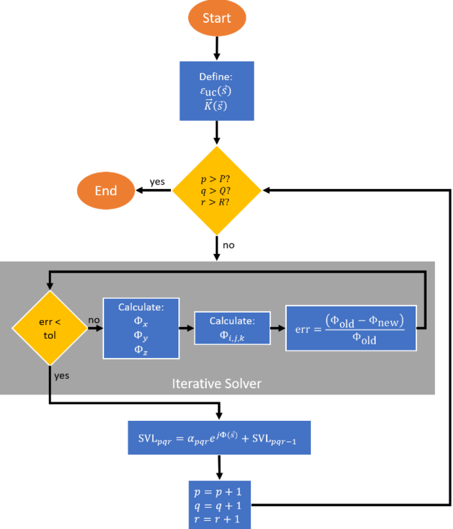
Figure 1: Flowchart describing the algorithm and its steps. The area inside of the gray box represents the iterative solver for the grating phase. A grating phase is calculated for every Cartesian direction and then combined into a singular global grating phase.

B. Algorithm inputs

In the first presentation of the algorithm to generate SVLs, Rumpf [5] described the most common inputs to the algorithm. The first input consists of the function representing the baseline periodic element that describes the lattice, ${\epsilon }_{uc}(\overrightarrow{s})$. In this paper, this function is set to 0 for all areas describing air and 1 for areas where material exists.

This baseline unit cell is then decomposed into a complex Fourier series via a fast Fourier transform (FFT). Each term in the Fourier series is a spatial harmonic with its own direction, amplitude, and period and, thus, can be considered as a single sinusoidal grating. ${\epsilon }_{uc}(\overrightarrow{s})$ then becomes a weighted sum of sinusoidal gratings of the form

$${\epsilon }_{uc}(\overrightarrow{s})=\sum _p^P\sum _q^Q\sum _r^R{\alpha }_{pqr}{e}^{j{\overrightarrow{K}}_{pqr}\overrightarrow{s}}.$$

(27)

where $\overrightarrow{s}$ is position, ${\alpha }_{pqr}$ is the complex Fourier coefficient of the $pq{r}^{th}$ term, and ${\overrightarrow{K}}_{pqr}$ is the grating vector associated with the $pq{r}^{th}$ term. The associated grating vectors are calculated analytically according to

$${\overrightarrow{K}}_{pqr}=p{\overrightarrow{T}}_1+q{\overrightarrow{T}}_2+r{\overrightarrow{T}}_3.$$

(28)

The second set of data in [11] consists of a series of functions that define the spatial variance of the lattice parameters. Separate functions for lattice spacing, fill fraction, and unit cell orientation need to be constructed that describe the intended behavior for the final lattice. The examples of input functions described in Figure 2 show a lattice orientation that changes based on the direction of a line path as well as the lattice spacing being spatially varied in a Gaussian profile to go from 0 to 1 of the nominal lattice spacing; finally, the fill fraction of the device is changed radially outward to go from 1% to 100%. It is important to note that these input maps can take any shape the end-user requires for their application. The examples in Figure 2 is a graphical representation of a subset of possible maps.

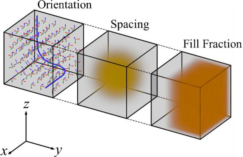
Figure 2: Sample algorithm inputs. From left to right: lattice orientation, lattice spacing, and lattice fill fraction. Any of these input maps can be drawn graphically on a Cartesian grid to represent arbitrary shapes.

C. Build spatially variant $\overrightarrow{K}$ function

To compute the spatially variant $\overrightarrow{K}$ function, an array that encompasses the problem space is constructed. The ${\overrightarrow{K}}_{pqr}$ grating vector associated with the $pq{r}^{th}$ spatial harmonic is extracted and applied to the whole grid. A rotation matrix is generated to aid in the addition of the tilt of the orientation to an intermediary $\overrightarrow{K}$ value at a point in the grid.

In order to calculate the spatially variant $\overrightarrow{K}$, the iterative solver shown in the flowchart in Figure 1 first needs to calculate the grating phase in accordance with eqn (3). The grating phase is solved iteratively in accordance with eqn (24)–(26), and at each iteration, ${\mathrm{\Phi }}_{\mathrm{old}}$ and ${\mathrm{\Phi }}_{\mathrm{new}}$ are compared to each other. This comparison is done to determine when the iteration process to calculate the grating phase stops. In this implementation, this criteria for stopping the iterative process is controlled by a tolerance factor; this means that once the numerical difference between ${\mathrm{\Phi }}_{\mathrm{old}}$ and ${\mathrm{\Phi }}_{\mathrm{new}}$ is negligible, the answer for the grating phase is considered complete.

D. Calculate spatially variant grating

After computing the overall grating phase throughout the problem space, the spatially variant grating, ${\epsilon }_{pqr}(\overrightarrow{s})$, is calculated with the use of

$${\epsilon }_{pqr}(\overrightarrow{s})={\alpha }_{pqr}{e}^{j{\mathrm{\Phi }}_{pqr}(\overrightarrow{s})}$$

(29)

where ${\alpha }_{pqr}$ represents the Fourier coefficient for the $pq{r}^{th}$ planar grating of the unit cell.

E. Calculate overall lattice

Having calculated each spatially variant grating, the overall lattice is obtained from their sum

$${\epsilon }_a(\overrightarrow{s})=ℝ\left[\sum _{pqr=1}^{PQR}{\epsilon }_{pqr}(\overrightarrow{s})\right]$$

(30)

The numerical noise caused by the use of the FFT and the construction of the lattice via the use of eqn (30) can cause the values in ${\epsilon }_a(\overrightarrow{s})$ to contain an imaginary component, which should be dropped by retaining only the real part of the summation.

III. GENERATION AND SIMULATION OF FULLY 3D SVLs

As mentioned in Section I, a potential application of SVLs is a spatially variant SCPC to direct the flow of light through a volume. The algorithm will be demonstrated here by generating and simulating this type of lattice. In the sections that follow, a technique for generating the input maps for this type of lattice is described. Then, two different spatially variant SCPC structures are generated with the iterative algorithm described in this paper. Finally, the results of an FDTD simulation of these structures are presented to demonstrate that functional lattices can be generated.

A. Line-path algorithm: An intuitive lattice orientation generator for SCPCs

This section describes the approach used to calculate the lattice orientation input map for flowing an electromagnetic wave around a double bend. The algorithm begins by creating a line path that the electromagnetic wave should follow. This is shown in Figure 3.

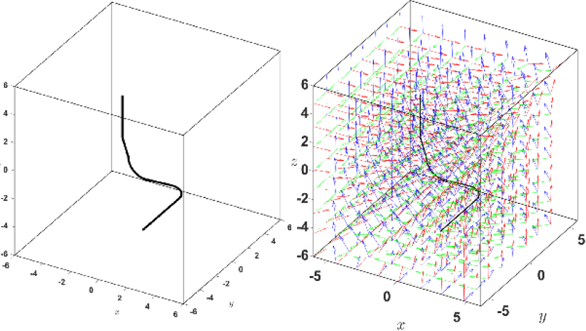
Figure 3: Line path used as nominal unit cell orientation (left) and the output lattice orientation (right). The figure on the left represents the nominal path an electromagnetic beam would follow inside of the lattice. The figure on the right represents the orientation vectors of each unit cell as a function of position based on the orientation line.

For each discrete point along the line, three vectors $\overrightarrow{a}$, $\overrightarrow{b}$, and $\overrightarrow{c}$ are defined that set the ideal orientation of the unit cells along the line. From here, the unit cell orientation of any other point within the lattice is set equal to the orientation defined at the closest point on the line. A loop is set up that iterates through every point in the lattice and calculates the three vectors $\overrightarrow{a}$, $\overrightarrow{b}$, and $\overrightarrow{c}$ for each point. The lattice orientation function that results from this process is shown in Figure 3.

B. Large lattice simulations

Two spatially variant SCPCs were generated from the two different unit cells, as shown in Figure 4. The unit cell in the left portion of Figure 4 is a simple cubic unit cell with the same dimensions and material parameters shown in [5]. The second lattice uses a hexagonal unit cell, as shown in the right portion of Figure 4, which exhibits broadband, omnidirectional, out-of-plane, and self-collimation as described in [12] . These structures were selected for generation with this algorithm due to their sensitivity to lattice spacing and overall structure [5, 12]. The final generated lattices are shown in Figure 5. In Figure 5, red arrows represent the input and output ports of the electromagnetic wave.

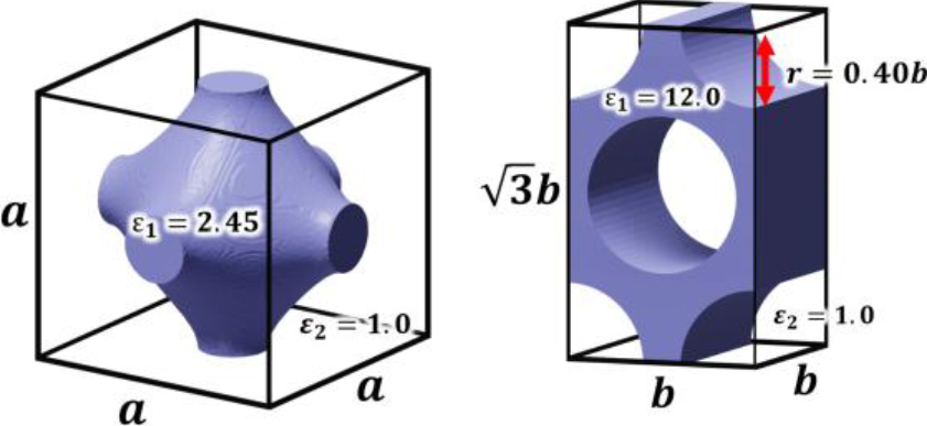
Figure 4: Unit cells used to generate the two spatially variant SCPCs with their respective materials and dimensions. Cubic unit cell (left) has dimensions $a$ = 1.59 cm and hexagonal unit cell (right) has dimensions $b$ = 1.00 cm.

Figure 5: Generated spatially variant SCPCs. The arrows show the input and output directions of the electromagnetic waves. Left generated with a cubic unit cell, total dimensions 20$a$ = 31.90 cm. Right generated with a hexagonal unit cell, total dimensions 12$b$ = 12.00 cm.

Full-wave simulations were performed using Remcom’s XFDTD software. The source used was a Gaussian beam that was linearly polarized along the z-axis impinging the input face of each self-collimating SCPC as shown in Figure 5. Each lattice was simulated at two difference frequencies and these were $f_1=15$ GHz and $f_2=22.5$ GHz. The beam inside of the lattice was expected to follow the orientation of the unit cells due to propagating through an SC crystal. Results for both the simple cubic and hexagonal spatially variant SCPCs are shown in Figures 6 and 7.

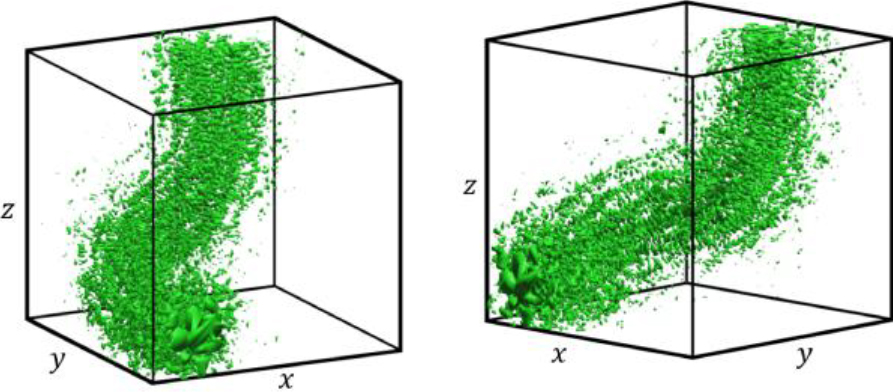
Figure 6: FDTD simulation of electric field intensity in a spatially variant lattice generated with a cubic unit cell at $f_1$ = 15 GHz with a Gaussian beam ($\omega$ = 2.985cm).

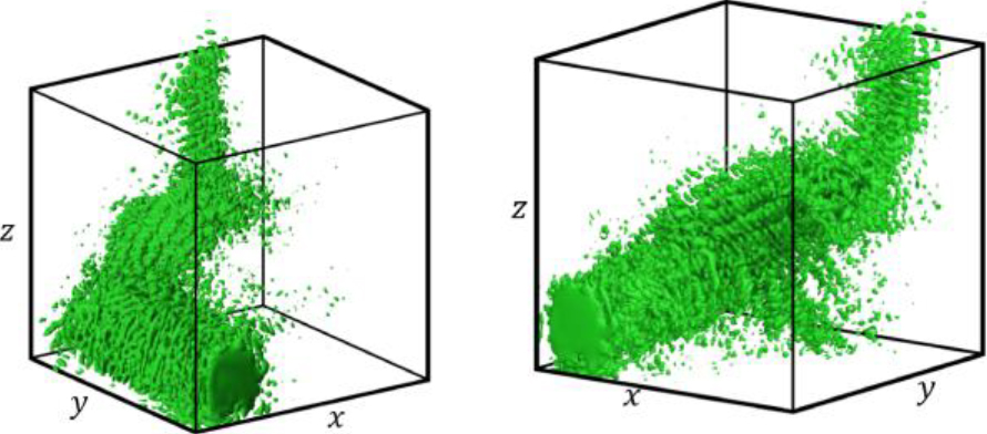
Figure 7: FDTD simulation of electric field intensity in a spatially variant lattice generated with a hexagonal unit cell at $f_2$ = 22.5 GHz with a Gaussian beam ($\omega$ = 1.333cm).

Both simulations shown in Figures 6 and 7 show the electromagnetic wave traveling through the lattice following the curvature defined in Figure 3 and exiting through the output face. The simulation shown in Figure 6 exhibits greater spurious scattering. There are two main reasons for this. First, the cubic unit cell has weaker self-collimation; so it has a limited range of angles, or field-of-view (FOV), in which a wave can self-collimate. The waves outside this FOV will scatter into different directions and will not follow the defined path of SC. Second, the lattice orientation function fed into the SV algorithm was not enforcing the vectors perpendicular to the direction of SC, and, thus, the unit cell orientation across the three axes of freedom was not enforced. This can further change or reduce the limited FOV of the unit cell, leading to unwanted scattering. It is hypothesized that the performance of the lattice with the cubic unit cell can be improved by enforcing all three axes of freedom to follow the curvature, along with a deformation control [13] algorithm to further suppress any deformations along the path. The simulation of the hexagonal unit cell shows much better performance with almost zero spurious scattering. The hexagonal unit cell exhibits omnidirectional SC along the main axis of propagation, allowing the beam to exit the intended output face with minimal scattering loss.

III. RESULTS

The algorithm was benchmarked against the matrix-based SVL computation approach for memory consumption. Figure 8 presents the results of the benchmark when the number of unit cells in a simple cubic lattice is increased in the $x$, $y$, and $z$ directions. These results were obtained by calculating the total memory space allocated inside of MATLAB® for the working variables of the grating phase, input maps, and intermediate parameters used in MATLAB’s LU decompositionalgorithm.

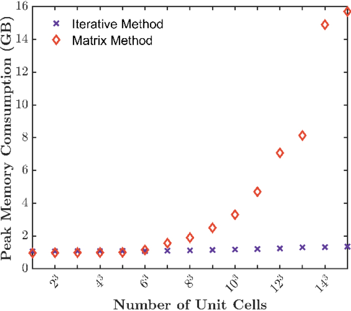
Figure 8: Iterative solver vs. matrix solver memory usage.

Figure 8 shows that there is a linear trend in the peak memory utilization while using the iterative SVL solver, whereas the peak memory usage when using the matrix solver shows an exponential growth. These trends in memory usage are a clear indication that the iterative solver presented is an excellent tool to generate large-scale lattices, while the matrix solver falls behind in memory consumption due to the computationally expensive LU decomposition.

III. CONCLUSION

It was shown that the formulation of an iterative SVL algorithm can be used to produce fully three-dimensional SVLs with greater memory efficiency. A line path algorithm was used to convey the unit cell orientation as a function of position in an easy and intuitive manner. Large-scale SVLs were able to be generated to be used in electromagnetic applications as spatially variant PhCs. Two lattices consisting of $20\times 20\times 20$ and $12\times 12\times 12$ unit cells, respectively, were generated and simulated using the FDTD method to confirm the device functionality. The low memory requirements of the iterative approach to generating SVLs allow for the realization of much larger photonic devices. Further, many geometrical properties in addition to unit cell orientation can be spatially varied to control multiple aspects of the wave at once in a 3D volume. This may prove valuable for unlocking the full potential that PhCs can offer to arbitrarily control electromagnetic waves throughout avolume.

ACKNOWLEDGMENT

Distribution A: Approved for public release - distribution unlimited (96TW-2021-0104)

REFERENCES

[1] H. Kosaka, T. Kawashima, A. Tomita, M. Notomi, T. Tatamura, T. Sato, and S. Kawakami, “Self-collimating phenomena in photonic crystals,” vol. 74, no. 9, pp. 1212-1214, 1999.

[2] M. Notomi, K. Yamada, A. Shinya, J. Takahashi, C. Takahashi, and I. Yokohama, “Extremely large group-velocity dispersion of line-defect waveguides in photonic crystal slabs,” Phys. Rev. Lett., vol. 87, no. 25, pp. 253902-253902-4, Dec.2001.

[3] R. C. Rumpf and J. Pazos, “Synthesis of spatially variant lattices,” Opt. Express, vol. 20, no. 14, pp. 15263, Jun. 2012.

[4] R. C. Rumpf, “Engineering the dispersion and anisotropy of periodic electromagnetic structures,” in Solid State Physics - Advances in Research and Applications, vol. 66, pp. 1212-1214,2015.

[5] R. C. Rumpf, J. Pazos, C. R. Garcia, L. Ochoa, and R. Wicker, “3D printed lattices with spatially variant self-collimation,” Prog. Electromagn. Res., vol. 138, pp. 1-14, 2013.

[6] J. L. Digaum, R. Sharma, D. Batista, J. J. Pazos, R. C. Rumpf, and S. M. Kuebler, “Beam-bending in spatially variant photonic crystals at telecommunications wavelengths,” Advanced Fabrication Technologies for Micro/Nano Optics and Photonics IX, vol. 9759, pp. 975911, 2016.

[7] J. J. Gutierrez, N. P. Martinez, and R. C. Rumpf, “Independent control of phase and power in spatially variant self-collimating photonic crystals,” J. Opt. Soc. Am. A, vol. 36, no. 9, pp. 1534-1539, 2019.

[8] K. David and C. Ward, Numerical analysis $\mathrm{|}$ mathematics $\mathrm{|}$ Britannica, 3rd ed. Pacific Grove: American Mathematical Sociecty, 2000.

[9] S. D. Gedney, “Introduction to the Finite-Difference Time-Domain (FDTD) Method for Electromagnetics,” Synth. Lect. Comput. Electromagn., vol. 6, no. 1, pp. 1-250, Jan. 2011.

[10] D. De Donno, a. Esposito, L. Tarricone, and L. Catarinucci, “Introduction to GPU Computing and CUDA Programming: A Case Study on FDTD [EM Programmer’s Notebook],” IEEE Antennas Propag. Mag., vol. 52, no. 3, pp. 116-122, 2010.

[11] R. C. Rumpf and J. Pazos, “Synthesis of spatially variant lattices,” Opt. Express, vol. 20, no. 14, pp. 15263-15274, 2012.

[12] Y. C. Chuang and T. J. Suleski, “Photonic crystals for broadband, omnidirectional self-collimation,” J. Opt., vol. 13, no. 3, pp. 1-8, 2011.

[13] R. C. Rumpf, J. J. Pazos, J. L. Digaum, and S. M. Kuebler, “Spatially variant periodic structures in electromagnetics,” Philos. Trans. R. Soc. A Math. Phys. Eng. Sci., vol. 373, no. 2049, p. 20140359, Jul. 2015.

ACES JOURNAL, Vol. 37, No. 2, 141–148.
doi: 10.13052/2022.ACES.J.370201
© 2021 River Publishers

Abstract

I. INTRODUCTION

II. GENERATION OF SPATIALLY VARIANT LATTICES

A. Spatially variant planar gratings and lattices

B. A general solution for $\nabla \mathrm{\Phi }(\overrightarrow{s})=\overrightarrow{K}(\overrightarrow{s})$

III. ITERATIVE SOLUTION TO $\nabla \mathrm{\Phi }(\overrightarrow{s})=\overrightarrow{K}(\overrightarrow{s})$

A. The update equation

B. Boundary conditions

III. IMPLEMENTATION

A. Algorithm flowchart

B. Algorithm inputs

C. Build spatially variant $\overrightarrow{K}$ function

D. Calculate spatially variant grating

E. Calculate overall lattice

III. GENERATION AND SIMULATION OF FULLY 3D SVLs

A. Line-path algorithm: An intuitive lattice orientation generator for SCPCs

B. Large lattice simulations

III. RESULTS

III. CONCLUSION

ACKNOWLEDGMENT

REFERENCES