Convolutional Neural Network for Array Size Selection of a Dual-band Reconfigurable Array
Garrett A. Harris, Corey M. Stamper, and Michael A. Saville
Department of Electrical Engineering
Wright State University, Dayton, Ohio, 45435, USA
michael.saville@wright.edu
Submitted On: April 15, 2022; Accepted On: April 13, 2023
ABSTRACT
A convolutional neural network (CNN) is designed and trained to partially control a dual-band, large uniform rectangular array of reconfigurable radiating elements. The CNN selects the number of active elements and switch states needed to achieve a desired beam shape. Both pattern multiplication and finite element method (FEM) are used to simulate the radiation patterns of a PIN-diode square-spiral antenna array. After training on radiation pattern images of arrays calibrated for both phase and gain imbalance and mutual coupling, the CNN achieves 97 percent validation accuracy. Then, using the resulting size and switch states, the patterns are simulated with and without mutual coupling using the pattern multiplication model and FEM, respectively. The mean beam steering and 3-dB beamwidth errors without mutual coupling are less than 5.5 degrees and up to 12.3 degrees with mutual coupling.
Index Terms: convolutional neural network, machine learning, pattern multiplication, reconfigurable array.
I. INTRODUCTION
Multichannel arrays are commonly used as multiple-input multiple-output (MIMO) antennas in communications [1–3] These antennas are essential for multi-beam forming [4], fast angle-of-arrival estimation [5], interference suppression [3], and array calibration [6–7]. The reconfigurable antenna has gained much attention for MIMO arrays because it can facilitate smart antenna technology in which the system senses the environmental conditions and automatically changes the antenna elements and circuitry to operate at different frequencies [2], with different polarization states [8], and with different radiation patterns [1, 9], or a combination thereof [10].
Typical switch methods [3] for the reconfigurable antenna include radio-frequency (RF) micro-electromechanical machines (MEMS), PIN diodes, and varactors, but emerging methods include liquid metals [12], plasma tubes [13], and laser-controlled optical windows [14]. Regardless of the type of switch, the reconfigurable array also requires careful treatment to minimize switch redundancy and to meet beam shape objectives [3]. The machine learning methods such as deep and convolutional neural networks [15–20] have gained much attention for such solutions.
For example, in [17], a 2D PIN-diode reconfigurable intelligent surface (RIS) is used to maximize bit rate in a MIMO system where a CNN is trained to learn the beamforming phases of the RIS for an arbitrary receiver direction. In [18], sidelobe level is controlled by particle swarm and bacteria foraging optimization and is shown to be effective even when individual elements fail. In [19], a CNN is used to design the required complex weights for an 8 8 planar array so that it can be steered in a desired direction. In a similar example, a multilayer perceptron network is trained in [20] to produce the complex beam steering weights for a uniform linear array of square patches. The recent work of [21] introduced a dual-CNN concept where the CNN estimates the required active elements and steering weights when given an arbitrary radiation pattern.
Prior to the recent popularity of CNNs, a great deal of research was done on using genetic algorithms to design array layouts. In [22], several genetics-inspired algorithms are presented to optimize widely-spaced, wideband arrays with a focus on minimizing sidelobe levels. Another article [23] explores the use of genetic algorithms to design highly directional and rotationally symmetric arrays. However, genetic algorithms require a large time commitment. In one example presented in [23], a single array design took over 270 hours to complete. This makes CNNs particularly attractive due to their ability to solve complex optimization problems in a matter of minutes rather than hours. However, array size selection for reconfigurable arrays have yet to be reported in the literature.
Most CNNs for arrays consider simple radiating elements such as patches, or are limited to a fixed and small array size. Here, we present a novel CNN that predicts the required number of active elements as well as antenna state of a large uniform reconfigurable rectangular array when given an arbitrary desired specification of beam direction and shape. The array element in this work consists of frequency and pattern reconfigurable spirals designed with the PIN diode single-turn square spiral antenna (PSSA) [24–25].
As it is well known how the CNN training relies on thousands of observations, the pattern multiplication model is used to generate radiation pattern images. The CNN is designed to select the array size and PIN diode ON/OFF states. Training with the images allows the CNN to learn the control parameters that meet a fully specified beam shape, i.e. main beam shape, sidelobe level, and null placement.
The paper is organized as follows: Section II describes the unit cell and array design of [24]. Section III presents the pattern multiplication model and the method to create training images. Section IV describes the CNN and its training. Results and conclusions are presented in Sections V and VI, respectively.
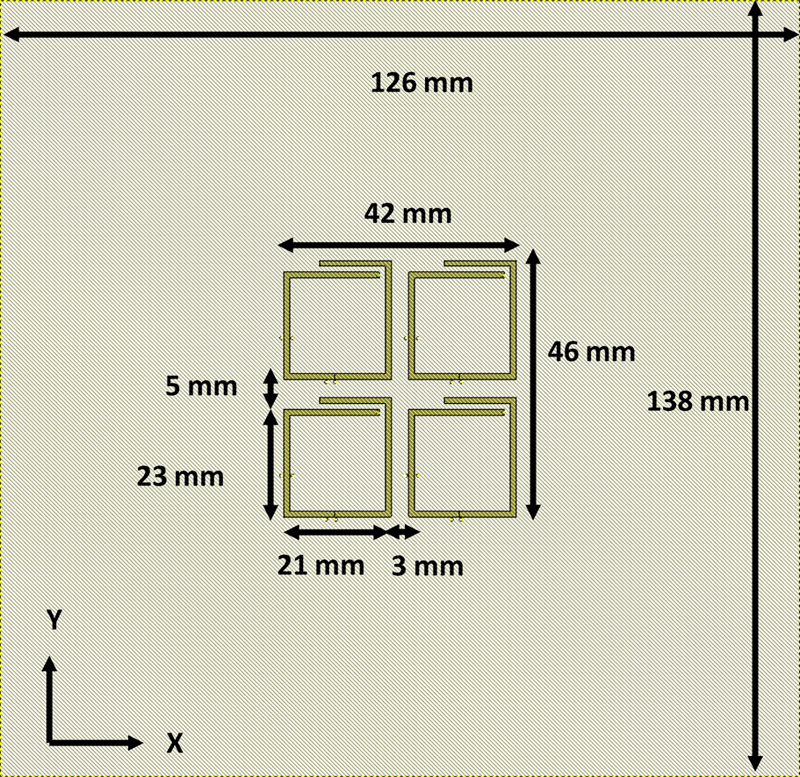
Figure 1: Layout of the unit cell of [24] but with a larger finite ground plane.
II. ANTENNA ARRAY
A. Reconfigurable element
For the communications array, we considered different reconfigurable antennas that operate at discrete frequencies, could be easily scaled and easily implemented. Hence, the printed square spiral, being in the class of frequency independent antennas, offers both wideband tuning and would easily scale during fabrication. The work of [25] presented a PSSA that used two PIN diodes: one series diode to change the frequency of operation from 3.75 GHz to above 6.0 GHz, and one shunt diode to change the radiation pattern from a boresight pattern to a squinted beam. Thus, the array could operate in two discrete bands (S and C). Also, the radiation pattern was considered for its potential to add an additional degree of freedom in digital beam shaping of the array, but was ultimately left unused. Lastly, the planar form of the PSSA could be arranged in a multichannel planar array where each unit cell has a dedicated transceiver for digital beamforming.
B. Unit cell and array
The planar array design of [24] defines the unit cell as a 2 2 rectangular arrangement of identical PSSA elements with elemental spacings d = 42.0 mm, and d = 46.0 mm as shown in Fig. 1. Using a five-layer layout for the model, based on two sheets of Roger’s Duroid 5880, the unit cells and feed network are on the top and bottom copper layers, respectively. Conductive vias connect the bias lines to the PIN diodes through the middle copper shielding layer.
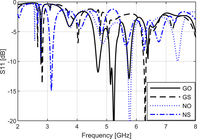
Figure 2: S11 of the unit cell for each switch state.
The design was modeled with Cadence AWR [24] software using a five-layer stack representing the dielectric laminates. The diode model uses ideal ON and OFF states as in [25] where the microstrip trace is continuous for the ON state and a gap is placed at the location of the diode for the OFF state. The gap length is equal to the physical size of the diode. As an alternative model, the diodes could have been replaced with microstrip transmission lines of equivalent S-parameters [2], or with a series resistor and capacitor [8]. We also note how the model lacks a DC blocking capacitor and RF choke which would affect the final antenna pattern. Differences with the simulated unit cell’s radiation pattern with and without the added components and lines are independent of the neural network training methodology and would only require an updated set of simulated radiation pattern images during training.
In the following, the switch state descriptions follow [25] as GO, GS, NO, and NS where O and S denote open (OFF) and short (ON) for the series diode, and G and N denote grounded (ON) and not grounded (OFF) for the shunt diode. The design in [24] also considered various rotations and reflections of the individual PSSA elements but found that the 2 2 uniform placement provided the best uniformity of the radiation patterns of the different states and was deemed most appropriate for a large array. The arrangement also made the layout simpler for the control lines and corporate feed line. Each PSSA element of the unit cell has one series and one shunt diode, both of which are enabled/disabled at the same time during operation. However, unlike [21], the ground plane for the unit cell used here is sized for a 3 3 array to provide better backlobe characterization.
The unit cell has subtle differences in frequency of operation and radiation pattern when compared to those of the single PSSA element with the same switch state. Figure 2 shows the S11 responses from 2.0 to 8.0 GHz. Table 1 lists the resonant frequencies used in this work along with the 10-dB bandwidths, and half-power beam widths for the radiation patterns shown in Fig. 3.
Table 1: Frequency, 10-dB bandwidth, and half-power beam width of the unit cell for each switch state
| NS | NO | GS | GO | |
| Frequency (GHz) | 3.10 | 5.80 | 6.30 | 5.23 |
| 10-dB bandwidth (MHz) | 60.0 | 150.0 | 80.0 | 190.0 |
| Az-HPBW (deg) | 180.0 | 180.0 | 76.0 | 64.0 |
| El-HPBW (deg) | 76.0 | 56.0 | 56.0 | 56.0 |
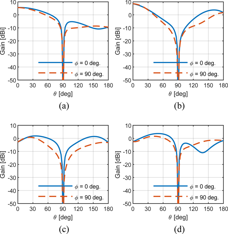
Figure 3: Gain pattern cuts in dBi of the unit cell for each switch state. Cuts along at = 0 deg. (solid line) and = 90 deg. (dashed line). (a) NS at 3.13 GHz. (b) NO at 5.78 GHz. (c) GS at 6.30 GHz. (d) GO at 5.24 GHz.
III. PATTERN MULTIPLICATION MODEL
A. Array pattern model
The pattern multiplication model is a well-known approximation of the array pattern and assumes the antenna elements have the same current distribution. The factored array pattern is
| (1) |
where is the unit cell’s radiation pattern and is the array factor. The model ignores mutual coupling and effects of a finitely sized array. However, it allows efficient calculation of the array pattern and study of the antenna performance in digital beamforming applications.
The unit cell of each reconfiguration state is first modeled with Cadence AWR software in the - plane, and the radiation pattern is simulated over the set of discrete spherical angles in degrees. However, the digital beamforming model is defined in the y-z plane with the azimuth and elevation angular coordinates shown in Fig. 4. Hence, the unit cell pattern is resampled using spline interpolation from the AWR reference frame to the array’s reference frame at aspects in degrees. This approach avoids beam wrapping in the radiation pattern image and the need to cast images in sine space coordinates [19].
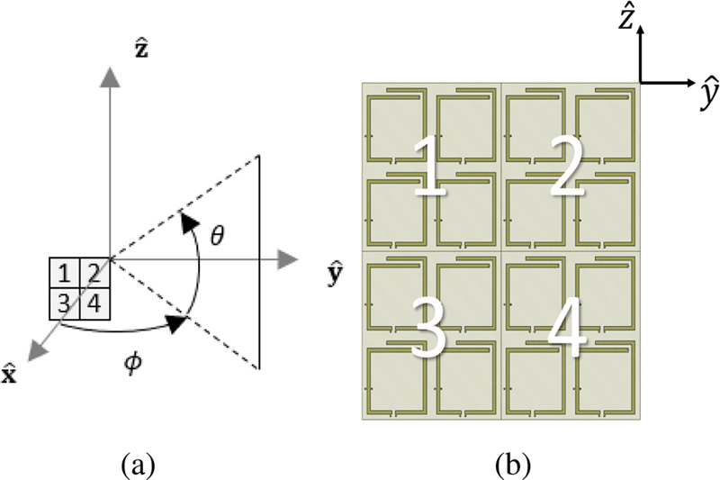
Figure 4: (a) Array reference frame. (b) Four unit cells showing the reference element.
Each unit cell has position where , and and are the elemental spacing. For the signal direction
| (2) |
the -th cell has phase:
| (3) |
which is relative to the reference element. In equation (3), is the wave number and the superscript denotes vector transpose.
For efficient calculation, the weighted array factor
| (4) |
is recast from the matrix-vector product in (4) to the steering vector product using:
| (5) |
where denotes the Kronecker vector product and:
| (6a) |
| (6b) |
In equation (5), the azimuth () and elevation () steering vectors represent the incremental phase progression across each dimension of the array. In equation (4), is the complex weight used to electronically control the beam direction and shape upon transmission. In a receive mode, it represents the signal from an arbitrary direction .
The weighted steering vector for beam steering in the direction with controlled sidelobes is:
| (7) |
where denotes the Hadamard vector product. The azimuth and elevation weight vectors control sidelobe levels with windowing functions such as Taylor and Hanning, etc. Therefore, the array’s radiation pattern in the direction is:
| (8) |
where the superscript denotes the Hermitian transpose.
B. Training data generation
Figure 5 shows the normalized intensity patterns for the different states of the unit cell for an 8 8 array. Each pixel in the image corresponds to a direction and the pixel value is calculated with equation (8). The weights of equation (7) are selected as 35-dB Taylor weights, and the beam is steered to boresight . Figure 6 shows the pattern when the beam is steered to elevation and azimuth .
The images of Figs. 5 and 6 are normalized intensity with units of decibels. In Section IV, equation (8) is used to create a single channel image representing linear gain scaled to [-1,1]. It is noted how an alternative approach and possibly a better approach is to use three-channel images where channel 1 is the normalized intensity image on a decibel scale with 60-dB dynamic range, channel 2 is a linear-scale image, and channel 3 is a quarter-power linear-scale image. Finally, each image channel would also be scaled to theinterval [-1,1].
C. Consideration of mutual coupling
The analysis of [24] considered effects of mutual coupling and concluded that the effect on the pattern multiplication model was negligible for arrays larger than 3 3. However, the GO and GS patterns showed a greater impact of mutual coupling than the NS and NO patterns. When the shunt diode is off, the current flow remains in the spiral winding and exhibits an overall symmetry about the unit cell. However, when the shunt diodes are on (GO,GS), a portion of the current flows to the ground plane and disturbs the symmetry. As reported in [25], the lack of symmetry changes the radiation pattern but also causes an increased contribution to mutual coupling.
Hence, the unit-cell pattern of equation (8) was simulated as an isolated 2 2 array of PSSA elements and designated as to distinguish it from the embedded unit cell pattern . The embedded pattern was simulated in AWR as a 3 3 array of unit cells with the center cell active and all others inactive. Both array patterns and are considered during the CNN training.
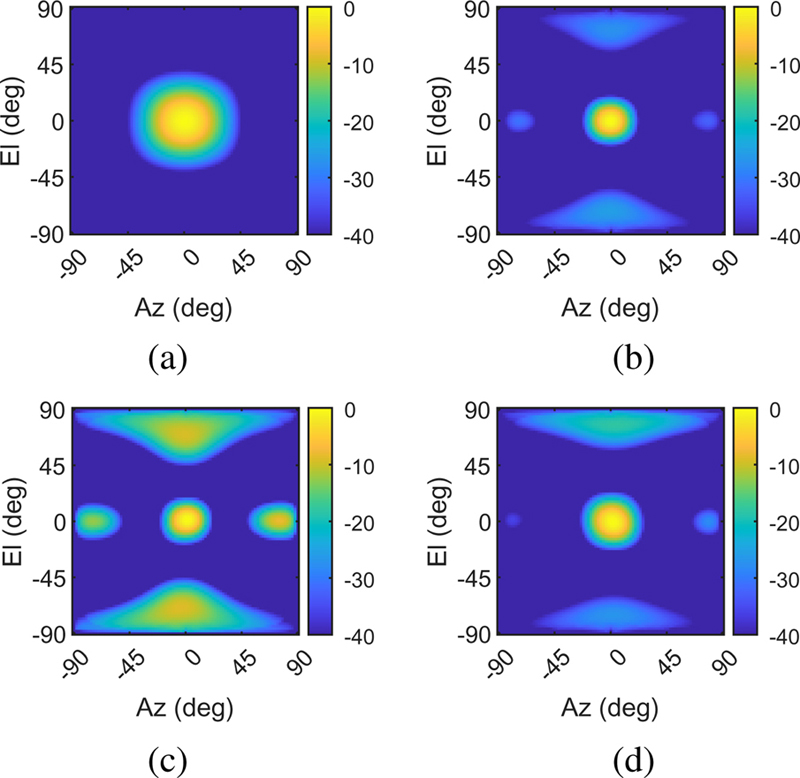
Figure 5: Normalized 3D gain patterns in dB for the array. The signal arrives from aspect . (a) NS. (b) NO. (c) GS. (d) GO.
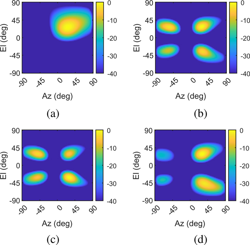
Figure 6: Normalized 3D gain patterns in dB for the array. The signal arrives from aspect . (a) NS. (b) NO. (c) GS. (d) GO.
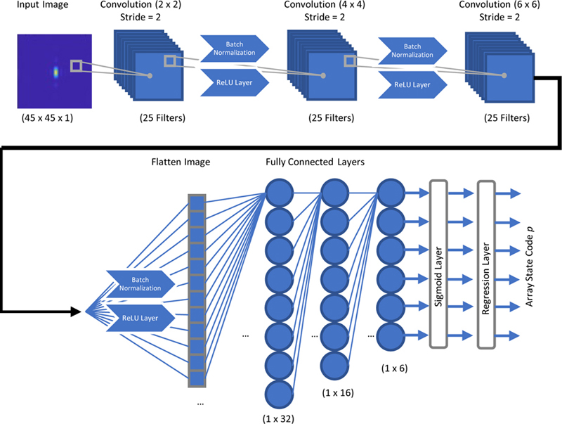
Figure 7: CNN architecture: the first stage comprises three convolution layers and the second stage consists of three fully connected input, hidden, and output layers.
IV. ARRAY CONFIGURATION WITH CNN
A. Machine learning approach
The general theories of CNN and machine learning are beyond the scope of this paper, but [26], [27] give the theory of the CNN, and for antenna array applications. The objective of the machine learning controller is to predict the length of each dimension of the array (,) and to predict the PIN diode switch states (NS,NO,GS,GO) that meet a desired array pattern. We assume that the unit cells are adjacent and have fixed spacing (). Then, we define the predicted array state vector as , which is cast as the binary number for convenience duringCNN training.
Unlike [15] that uses a self-organizing map neural network to learn the PIN diode switch states from 1D S11 data, we use a CNN to learn the relationship between the array pattern and . Our approach is similar to [19] where a CNN is trained to learn the phase control of an 8 8 planar array from 2D images of radiation patterns. Using equation (8), we generate a large sample of images for different array sizes and switch states and train a CNN to learn the relationship between the array pattern and the switch state when the beam is steered in an arbitrary direction. When simulating patterns with equation (8), the array is assumed to have ideal phase and gain calibration and ideal compensation for mutual coupling. Then, we use the trained CNN to predict the array state vector from an intensity image of the desired array pattern; that is, a mask of the pattern we want to radiate with the array.
There are two main challenges for using a CNN. First, training the CNN requires a large amount of data. Full-wave simulations would take an untenable amount of time so we use the pattern multiplication technique. Second, the neural network architecture is an art and requires substantial trial and error. Neural networks can have many different layers which all perform different tasks. Some layers work well together, and some do not. Next, we describe the training and testing data and the CNN architecture. We present results in Section V.
B. Training data
The input data consists of 46 46-pixel grayscale images that represent the magnitude of the radiation patterns in the forward hemisphere of the array. The set of images are generated with equations (7) and (8) using a variable array shape, reconfigurable switch state, and steering direction, which are represented in the label . We also scaled the pixel values to the interval [-1,1]. The length of the array in each dimension is allowed to be within [2, 4, 6, 8], and the steering direction is constrained to a 45-degree cone relative to boresight. Also, a 35-dB Taylor window is used to reduce sidelobes. Each image has dimensions corresponding to the azimuth and elevation angles of the forward hemisphere ofthe array.
For each combination of array size and switch state the array is steered to 1,000 uniformly sampled directions, and the total data set comprises 64,000 unique images. Lastly, 10 percent of the training data is randomly selected for use during CNN validation. This validation set comprises 6,400 images randomly selected before training. These images are not included in the training set but are used to estimate CNN accuracy after training. Validation accuracy during training is calculated as root mean square error (RMSE) from the known and predicted values of during training. In addition, the validation set was tested by calculating he percentage of correctly predicted state vectors.
C. CNN architecture
Figure 7 shows the CNN design that consists of a three-layer convolution stage followed by a three-layer neural network. In the first stage, each image is downsampled and then processed with eight 3 3 convolution kernels. The subsequent convolution layers use 5 5 and 7 7 kernels. Then, the images are flattened (vectorized) as input to the neural network. Three hidden layers are used. The output of the CNN is quantized as 0 or 1 in order to create a binary number that represents the array state. Table 2 lists the specific layers, convolution window sizes, and number of nodes. Table 3 lists the final set of hyperparameters that control batching, dropout, learning rate and loss metric. The output layer represents regression-based prediction of the array state but in a binary form. The specific CNN architecture was learned by trial and error [21]. Training the CNN on a Windows 10 machine with MATLAB 2021b took approximately 25 minutes on a single CPU (Intel i5 with 16 GB RAM), and 3 minutes on an Intel i7 with 32 GB with a single GPU (Nvidia RTX A3000 with 6GB).
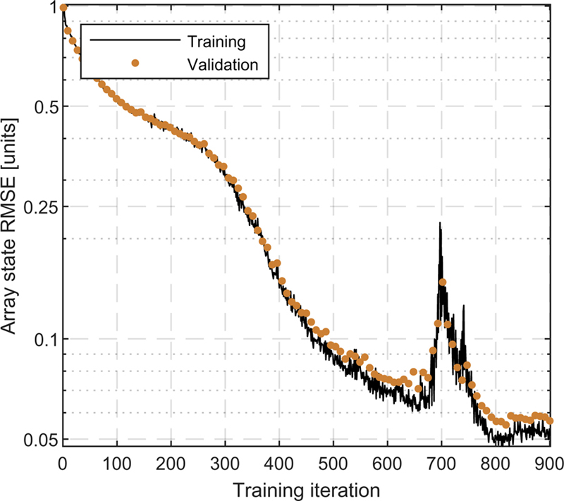
Figure 8: Root mean square error (RMSE) calculated with the known and predicted values of during CNNtraining.
V. RESULTS
After experimenting with several architectures and training schemes, the network achieved an accuracy of 97% on the validation data. This high level of accuracy indicates that the network learned the general relationship between the radiation patterns and the array configurations. However, we set up testing data to observe how well the network performs when given a radiation mask that was produced by a different method.
Hence, test data consists of arbitrary and novel radiation patterns (masks) that were unobserved by the CNN during training. We first generated masks with a 2D Gaussian pulse to approximate the main beam of the array for a desired beam direction and beamwidth. The network struggled to predict the correct array state for this mask type. Instead, we used Taylor-windowed isotropic array patterns using equations (5) and (7) and saw a noticeable improvement in validation accuracy. We considered how the sidelobe structure contributes to the CNN learning, and we confirmed it by observing how the respective neurons became active when null features were detected in the convolution layers.
Table 2: CNN layers characterized according to their function; e.g. convolution, batching, normalization, activation function, and connectedness
| Layer | Type | Options |
|---|---|---|
| Layer 1 | 2D Convolution | 25 22 Filters, Stride = 2 |
| Layer 2 | Batch normalization | n/a |
| Layer 3 | ReLU | n/a |
| Layer 4 | 2D Convolution | 25 44 Filters, Stride = 2 |
| Layer 5 | Batch normalization | n/a |
| Layer 6 | ReLU | n/a |
| Layer 7 | 2D Convolution | 25 66 Filters, Stride = 2 |
| Layer 8 | Batch normalization | n/a |
| Layer 9 | ReLU | n/a |
| Layer 10 | Fully connected | 32 Nodes |
| Layer 11 | Fully connected | 16 Nodes |
| Layer 12 | Fully connected | 6 Nodes |
| Layer 13 | Sigmoid | n/a |
| Layer 14 | Regression | n/a |
Table 3: CNN training options and hyperparameters that control the learning accuracy
| Hyperparameter | Setting |
|---|---|
| Optimization method | adam |
| Epochs | 100 |
| Mini batch size | 160 |
| Learning rate | 0.001 |
| L2 regularization | 0.001 |
| Gradient threshold | Inf |
In order to test the effectiveness of the CNN, 1,000 arbitrary radiation pattern masks were simulated for array sizes N,N in [2, 4, 6, 8] and main beam directions [-45 , 45] deg. The operating frequency was randomly assigned to one of the four unit cell frequencies listed in Table 1.
As the CNN returns a discrete array state p (size and switch configuration), we tested the effectiveness of the network’s prediction by comparing the pattern G(p) calculated with equation (8) to the input mask. For each test and mask pair we compared the mainlobe’s steering angles (,) and half-power beamwidths (,) and calculated the mean differences (, , ,) listed in Table 4. Except for the elevation steering angle which has a mean error of 5.5 deg., the mean error is less than 4 deg. and suggests the CNN has successfully learned the relationship between the pattern features and the array configuration. The increased error in the elevation steering angle is likely a result of the specific pattern of the unit cell. We also noticed how the beamwidth and steering angles were less than 2 degrees when the size of the array exceeded 33 and the steering angle was within a 30-deg. cone.
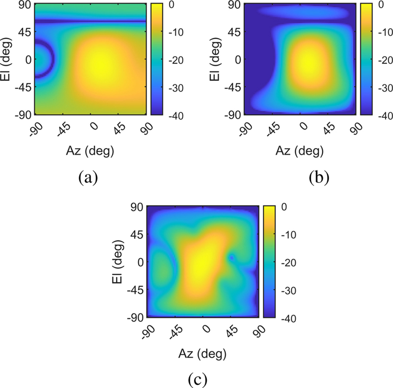
Figure 9: Desired and predicted patterns for beam steered to deg. and deg. Azimuth and elevation, respectively. (a) Desired pattern and CNN predictions using (b) and (c) .
The pattern when calculated with assumes ideal phase and gain calibration for the individual transmit and receive channels and ideal compensation for mutual coupling. To check the effects of mutual coupling, we selected several predicted array states where had errors less than 5 deg. and simulated the array pattern with AWR as . Thus, assumes ideal phase and gain calibration of the individual channels but no compensation for mutual coupling (MC). For computing time and memory limitations, only six array configurations were selected and the number of unit cells was limited to nine or less. Figures 9 shows an example with and steering angles of 17 deg. in elevation and 11 deg. in azimuth. Figures 9 (a) shows the test mask (windowed, isotropic array factor), Figs. 9 (b) shows (windowed, pattern multiplication model with ideal phase/gain calibration and MC-compensation), and Figs. 9 (c) shows (windowed, calibrated phase/gain, MC-uncompensated). The mean errors for are listed in Table 4, and are larger than the errors of .
Table 4: Mean steering angle and half-power beamwidth errors in degrees for pattern multiplication () and FEM () test images
| Test Method | ||||
|---|---|---|---|---|
| 5.5 | 3.7 | 2.9 | 2.7 | |
| 9.3 | 12.3 | 12.3 | 2.3 |
We effectively trained the CNN with patterns of a calibrated and MC-compensated array, but we tested with MC-uncompensated array patterns. The increase in error is reasonable given the well-known degrading effects of mutual coupling on the array pattern.
VI. CONCLUSION
A convolutional neural network has been presented for predicting the array state from an arbitrary beam shape. The network was trained with images of different radiation patterns and learned the number of elements needed to achieve the mask. Using a recently studied uniform rectangular array of reconfigurable planar square spiral antennas, the network achieved a 97% training accuracy. When tested with masks of different distributions than those used during training, the desired mask and the pattern multiplication model had good agreement between the beamwidths (less than 3 deg.) and steering direction (less than 6 deg.). However, when the mask was compared to the array pattern when mutual coupling was present, the errors increased by up to 12.3 degrees.
The CNN was trained using patterns representing the ideal case where there is no mutual coupling, and with balanced gain and phase. Future work will train CNNs with gain and phase imbalances as well as pattern distortions from mutual coupling in order to compensate for these limitations in real arrays.
ACKNOWLEDGMENT
The authors thank the DAGSI Fellowship program for supporting the foundational work presented in [24], and the DoD SMART Scholarship program for support during the current work.
REFERENCES
[1] Y. Zhou, R. S. Adve, and S. V. Hum, “Design and evaluation of pattern reconfigurable antennas for MIMO applications,” IEEE Trans. Antennas Propag., vol. 62, no. 3, pp. 1084-1092, doi: 10.1109/TAP2013. 2284874, Mar. 2014.
[2] D. Piazza, N. J. Kirsch, A. Forenza, R. W. Heath, and K. R. Dandekar, “Design and evaluation of a reconfigurable antenna array for MIMO systems,” IEEE Trans. Antennas Propag., vol. 56, no. 3, pp. 869-881, doi: 10.1109/TAP.2008.916908, Mar. 2008.
[3] Y. Tawk, J. Constantine, and C. G. Christodoulou, Antenna Design for Cognitive Radio, Artech House, Norwood, MA, 2016.
[4] L. Di Palma, A. Clemente, L. Dussopt, R. Sauleau, P. Potier, and P. Pouliguen, “Radiation pattern synthesis for monopulse radar applications with a reconfigurable transmitarray antenna,” IEEE Trans. Antennas Propag., vol. 64, no. 9, pp. 4148-4154, doi: 10.1109/TAP.2016.2586491, Sep. 2016.
[5] X. Wang, E. Aboutanios, M. Trinkle, and M. G. Amin, “Reconfigurable adaptive array beamforming by antenna selection,” IEEE Trans. Signal Process., vol. 62, no. 9, pp. 2385-2396, doi: 10.1109/TSP.2014. 2312332, May 2014.
[6] Y. Ji, J. Ø. Nielsen, and W. Fan, “A simultaneous wideband calibration for digital beamforming arrays at short distances [Measurements Corner],” IEEE Antennas Propag. Mag., vol. 63, no. 3, pp. 102-111, June 2021.
[7] T. W. Nuteson, J. E. Stocker, J. S. Clark, D. S. Haque, and G. S. Mitchell, “Performance characterization of FPGA techniques for calibration and beamforming in smart antenna applications,” IEEE Trans. Microw. Theory Tech., vol. 50, no. 12, pp. 3043-3051, doi: 10.1109/TMTT. 2002.805151, Dec. 2002.
[8] V. Zarei, H. Boudaghi, M. Nouri, and S. A. Aghdam, “Reconfigurable circular polarization antenna with utilizing active devices for communication systems,” Applied Computational Electromagnetics Society (ACES) Journal, vol. 30, no. 9, pp. 990-995, https://journals.riverpublishers.com/index.php/ACES/article/view/10395, Sep. 2015.
[9] H. Moghadas, M. Zandvakili, D. Sameoto, and P. Mousavi, “Beam-reconfigurable aperture antenna by stretching or reshaping of a flexible surface,” IEEE Antennas Wireless Propag. Lett., vol. 16, pp. 1337-1340, doi: 10.1109/LAWP.2016.2633964, Dec. 2016.
[10] L. Di Palma, A. Clemente, L. Dussopt, R. Sauleau, P. Potier, and P. Pouliguen, “Circularly-polarized reconfigurable transmitarray in Ka-band with beam scanning and polarization switching capabilities,” IEEE Trans. Antennas Propag., vol. 65, no. 2, pp. 529-540, doi: 10.1109/TAP.2016. 2633067, Feb. 2017.
[11] W. Li, L. Bao, and Y. Li, “A novel frequency and radiation pattern reconfigurable antenna for portable device applications,” Applied Computational Electromagnetics Society (ACES) Journal, vol. 30, no. 12, pp. 1276-1285, https://journals.riverpublishers.com/index.php/ACES/article/view/10291, Dec. 2015.
[12] A. M. Morishita, C. K. Y. Kitamura, A. T. Ohta, and W. A. Shiroma, “A liquid-metal monopole array with tunable frequency, gain, and beam steering,” IEEE Antennas Wireless Propag. Lett., vol. 12, pp. 1388-1391, doi: 10.1109/LAWP.2013.2286544, Oct. 2013.
[13] O. A. Barro, M. Himdi, and O. Lafond, “Reconfigurable radiating antenna array using plasma tubes,” IEEE Antennas Wireless Propag. Lett., vol. 15, pp. 1321-1324, doi: 10.1109/LAWP.2015.2507066, 2016.
[14] I. F. da Costa, A. Cerqueira S., D. H. Spadoti, L. G. da Silva, J. A. J. Ribeiro, and S. E. Barbin, “Optically controlled reconfigurable antenna array for mm-wave applications,” IEEE Antennas Wireless Propag. Lett., vol. 16, pp. 2142-2145, doi: 10.1109/LAWP. 2017.2700284, May 2017.
[15] A. Patnaik, D. Anagnostou, C. G. Christodoulou, and J. C. Lyke, “Neurocomputational analysis of a multiband reconfigurable planar antenna,” IEEE Trans. Antennas Propag., vol. 53, no. 11, pp. 3453-3458, doi: 10.1109/TAP.2005.858617, Nov. 2005.
[16] F. Zardi, P. Nayeri, P. Rocca, and R. Haupt, “Artificial intelligence for adaptive and reconfigurable antenna arrays: a review,” IEEE Antennas Propag. Mag., vol. 63, no. 3, pp. 28-38, doi: 10.1109/MAP.2020.3036097, June 2021.
[17] B. Sheen, J. Yang, X. Feng, and M. M. U. Chowdhury, “A deep learning based modeling of reconfigurable intelligent surface assisted wireless communications for phase shift configuration,” IEEE Open J. Commun. Soc., vol. 2, pp. 262-272, doi: 10.1109/OJCOMS.2021.3050119, Jan. 2021.
[18] O. P. Acharya, A. Patnaik, and S. N. Sinha, “Comparative study of bio-inspired optimization techniques in antenna array failure compensation,” in Proc. IEEE Int. Symp. Antennas Propag. (APSURSI), Orlando, FL, USA, pp. 1232-1233. doi: 10.1109/APS.2013. 6711276, 2013.
[19] R. Lovato and X. Gong, “Phased antenna array beamforming using convolutional neural networks,“ in IEEE Int. Symp. Antennas Propagat. and USNC-URSI Radio Science Meeting, Atlanta, GA, USA, pp. 1247-1248. doi: 10.1109/APUSNCURSINRSM.2019. 8888573, 2019.
[20] J. H. Kim and S. W. Choi, “A deep learning-based approach for radiation pattern synthesis of an array antenna,” IEEE Access, vol. 8, pp. 226059–226063, doi: 10.1109/ACCESS.2020. 3045464, Dec. 2020.
[21] G. A. Harris, “Reconfigurable array control via convolutional neural networks,” M.S. Thesis, Dept. Elect. Eng., Wright State Univ., Dayton, OH, 2021.
[22] D. H. Werner, M. D. Gregory, and P. L. Werner, “A review of high performance ultra-wideband antenna array layout design,” in 8th Eur. Conf. Antennas Propag. (EuCAP 2014), The Hague, Netherlands, pp. 3128-3131, doi: 10. 1109/EuCAP .2014.6902490, 2014.
[23] M. D. Gregory, F. A. Namin, and D. H. Werner, “Exploiting rotational symmetry for the design of ultra-wideband planar phased array layouts,” IEEE Trans. Antennas Propag., vol. 61, no. 1, pp. 176-184, doi: 10.1109/TAP .2012.2220107, Jan. 2013.
[24] C. M. Stamper, “Reconfigurable antenna array using the PIN-diode-switched printed square spiral element,” M.S. Thesis, Dept. Elect. Eng., Wright State Univ., Dayton, OH, 2021.
[25] G. H. Huff, J. Feng, S. Zhang, and J. T. Bernhard, “A novel radiation pattern and frequency reconfigurable single turn square spiral microstrip antenna,” IEEE Microw. Wireless Compon. Lett., vol. 13, no. 2, pp. 57-59, doi: 10.1109/LMWC.2003. 808714, Feb. 2003.
[26] I. Goodfellow, Y. Bengio, and A. Courville, Deep Learning, MIT Press, Cambridge, MA, 2016.
[27] M. Martinez-Ramon, A. Gupta, and J. L. Rojo-Álvarez, Machine Learning Applications in Electromagnetics and Antenna Array Processing, Artech House, Norwood, MA, 2020.
BIOGRAPHIES

Garrett A. Harris received his B.S.E.E. at Wright State University in 2020 and the M.S.E.E degree in 2022 via the DoD SMART scholarship. While a student he was a member of IEEE and an adviser for the Ohio Mu chapter of Tau Beta Pi. Garrett has spent two summers at Wright State’s Autonomy Technology Research Center internship with AFRL. His research interests include antenna design, remote sensing, and machine learning.
Corey M. Stamper received the B.S.E.E degree at Wright State University in 2020 and the M.S.E.E degree in 2021, also from Wright State University. His research interests are in applied electromagnetics, antenna design, and signal processing.
Michael A. Saville received the B.S.E.E., M.S.E.E., and Ph.D. degrees from Texas A&M University in 1997, the Air Force Institute of Technology in 2000, and the University of Illinois at Urbana-Champaign in 2006, respectively. He is currently Associate Professor of Electrical Engineering at Wright State University with a broad range of research interests in applied electromagnetics and applied signal processing. He is a Senior Member of IEEE, a registered Professional Engineer in Ohio, and Associate Editor for PIER Journal and IET Electronics Letters.
ACES JOURNAL, Vol. 38, No. 6, 400–408
doi: 10.13052/2023.ACES.J.380604
© 2023 River Publishers