Bayesian Optimization Based on Student’s T Process for Microstrip Antenna Design
Qing Li1, Fei Meng2, Yubo Tian3, and Xiaoyan Wang4
1Ocean College, Jiangsu University of Science and Technology, Zhenjiang 212003, China
leo199808@163.com
2School of Information and Communication Engineering, Guangzhou Maritime University, Guangzhou 510725, China
mengfei@gzmtu.edu.cn
3School of Information and Communication Engineering, Guangzhou Maritime University, Guangzhou 510725, China
tianyubo@just.edu.cn
Corresponding to Yubo Tian, Qing Li, and Fei Meng are co-first authors.
4Ocean College, Jiangsu University of Science and Technology, Zhenjiang 212003, China
1836351293@qq.com
Submitted On: April 18, 2022; Accepted On: September 3, 2022
Abstract
Bayesian Optimization (BO) is an efficient global optimization algorithm, which is widely used in the field of engineering design. The probabilistic surrogate model and acquisition function are the two keys to the algorithm. Building an efficient probabilistic surrogate model and designing a collection function with excellent exploring capabilities can improve the performance of BO algorithm, allowing it to find the optimal value of the objective function with fewer iterations. Due to the characteristics of small samples and non-parametric derivation of the Gaussian Process (GP), traditional BO algorithms usually use the GP as a surrogate model. Compared with the GP, the Student’s T Process (STP) retains the excellent properties of GP, and has more flexible posterior variance and stronger robustness. In this paper, STP is used as the surrogate model in BO algorithm, the hyperparameters of the model are optimized by STP, and the estimation strategy function (EST) is improved based on the posterior output of the optimized STP, thus realizing the improved BO algorithm based on the STP. To verify the performance of the proposed algorithm, numerical experiments are designed to compare the performances of the traditional BO algorithm, which includes the lower confidence bound function (LCB) and EST as acquisition function respectively and GP as the surrogate model, and the proposed BO algorithm with STP as the surrogate model and LCB, expected improvement function (EI), expected regret minimization function (ERM) as acquisition function respectively. The results show that the proposed algorithm in this paper performs well when finding the global minimum of multimodal functions. Based on the developed algorithm in this paper, the resonant frequency of printed dipole antenna and E-shaped antenna is modeled and optimized, which further confirms the good design ability and design accuracy of the BO algorithm proposed in this paper.
Index Terms: acquisition function; antenna optimization; Bayesian optimization; Gaussian process; Student’s T process
1 INTRODUCTION
Constructing efficient global optimization algorithms has always been the focus of research topic. As an advanced and efficient global optimization algorithm, the Bayesian optimization (BO) algorithm has received extensive attention and research [1]. The BO algorithm is a kind of acquisition function and surrogate model as its cores to fit the objective function, collecting new sample observations to achieve fast iteration and find the maximum or minimum value of the objective function [2].
In recent years, the research on the BO algorithm is inseparable from three aspects: the establishment of a new surrogate model [3], the optimization of the surrogate model [4], and the design of the acquisition function [5]. The performance of BO algorithms can be improved by constructing efficient surrogate models, such as random forests surrogate models [6], making multiple decision trees to improve computational efficiency and accuracy, and deep neural network surrogate models [7] to improve the model’s ability to handle large-scale data. In recent years, the optimization of surrogate models in BO algorithms has also become a research hotspot. Chowdhury [8] proposed a scheme to dynamically adjust the domain boundary of the surrogate model to solve the complex problem of high-dimensional data analysis. Yenicelik [4]designed an algorithm named BORING to deal with the dimensionality reduction of data. The acquisition function in parallel BO can collect multiple sample points simultaneously to improve its efficiency. Ginsburg et al. [9] studied Monte Carlo to simulate the acquisition function to generate multiple sample points at a time. Some scholars [10] also use the multimodal method to solve multiple candidate sample points, reducing the time-consuming problem of the simulation.
As a classical surrogate model in BO, Gaussian Process (GP) has a rigorous mathematical theoretical foundation and can deal with complex problems [11, 12]. However, GP has two apparent shortcomings. Its posterior variance depends on the observed sample points, and its outliers are based on a prior assumption, which makes GP not very good at rejecting outlier ability. Student’s T Process (STP) is a generalization of the GP, which obeys the Student’s T distribution rather than the Gaussian distribution [13]. The study of STP makes up for the lack of robustness of GP, and it has a more flexible posterior variance. Shah [14] proposed to perform the inverse Wishart process on the kernel function of the GP to realize the STP and use it to deal with outliers in the data. This is because the kurtosis of the Student’s T distribution is higher than that of the Gaussian distribution, which means it can contain outliers. More likely.
Särkkä [15] uses an STP instead of a GP and incorporates the noise term into the kernel function to simplify the computation. Tang et al. [16] proposed that when the input has noise that depends on the Student’s T distribution, if the kernel function does not have the property, the STP has a better ability to handle abnormal data. Chen et al. [17] proposed a multi-output GP and a multi-output STP, which solved the multi-output problem under the matrix variable of the STP. An effective way of improving the prediction accuracy and enhancing the performance of the model is to optimize the model’s hyperparameters. For example, the gradient descent method [18], particle swarm optimization algorithm [19], and ant colony algorithm [20] are used to optimize the super parameters of the nonparametric model, so as to improve the performance of the model.
Scholars have also studied the combination of STP and BO algorithm. In 2013, Shah [21] implemented the Bayesian algorithm using STP and the expected improvement function, and compared it with the Bayesian algorithm using the GP as a surrogate model for the function optimization problem. In 2018, Tracey [22] implemented the Bayesian algorithm combining the STP and the expected improvement function, and applied it to the design of aerodynamic structures. In 2020, Clare [23] used the improved expected regret minimization function and confidence bound minimization function, respectively, to combine with STP to form a new Bayesian algorithm, enhancing the ability of BO.
As we all know, the optimization of electromagnetic devices through full-wave electromagnetic simulation software requires enormous computing resources, which is very time-consuming. Therefore, exploiting optimizing algorithms to design electromagnetic devices quickly is a good solution [24]. Gao [25] proposed a semi-supervised algorithm for antenna design, but this algorithm requires an additional round of antenna size. Torun [26] designed a two-stage BO algorithm and applied it to the minimization optimization of integrated circuits, and the surrogate model used in this algorithm is the GP model.
In this paper, a BO algorithm is proposed, which uses the combination of an improved maximum evaluation policy function [27] and a hyperparameter-optimized STP. Moreover, it is applied to optimize multimodal functions, printed dipole antenna, and E-shaped antenna. The results show that the proposed BO algorithm has better exploration and global optimization abilities than the traditional BO algorithm.
The rest of the paper is organized as follows. The second part briefly reviews the derivation of GP and STP. The third part cover the proposed BO algorithm, including the hyperparameters for the STP, optimization and improvement of the maximum evaluation policy function. The fourth part is the numerical experiment, which verifies the performance of the proposed algorithm. The fifth part is the application of the proposed algorithm to two microstrip antennas, including printed dipole antenna and E-shaped antenna. The subsequent parts is the summary and outlook.
2 BACKGROUND
2.1 Gaussian process
Gaussian Process (GP), as a non-parametric model being suitable for small sample, has strict mathematical theoretical derivation. Generally, we use (1) to describe the GP [28, 29]:
| (1) |
where the is the mean function and the is the covariance function. If represents the observed set, then the covariance matrix K is recorded as:
| (2) |
For each input new observation , assuming that the mean of the GP is zero, the joint Gaussian distribution of the outputs and can be expressed as:
| (3) |
Where, is the covariance matrix of the order between the observation value and the training input samples, and is the covariance matrix of the observation value itself.
The posterior probability is obtained by calculating formula (4):
| (4) |
Here:
| (5) |
| (6) |
The GP can fit the corresponding test output value by calculating the above Process. It can be seen from equation (6) that the posterior variance of the GP depends on the test sample points. In BO, the acquisition function can use the information of the predicted mean and predicted variance of the GP to mine the next observation with high reliability. The acquisition function is introduced in Section 3.1.
2.2 Student’s T process
Student’s T Process (STP) is a generalization of GP, which refers to a functional distribution of an infinite set of random variables that obeys the joint Student’s T distribution. For the Student’s T distribution, we describe it as [18]:
| (7) | |||
where is the size of the T distribution, is the position parameter of the T distribution, is the symmetric positive definite scattering matrix parameter of the T distribution, and is the degree of freedom.
| (8) |
STP is parameterized by the mean function and the covariance function ; however, it has an additional parameter, the degrees of freedom . The properties of STP can be determined jointly by , and , is an arbitrary random variable. Therefore, STP can be expressed as:
| (9) |
With increasing degrees of freedom, the multivariate Student’s T distribution converges to a multivariate Gaussian distribution with the same mean, and the scattering parameter matrix approaches infinity.
In STP, defines the prior expected value of each location, the kernel function represents the covariance of the objective function between the values of any two locations and , the joint distribution probability of a finite subset of locations is:
| (10) |
Where is the mean vector, , is the kernel matrix.
Given a set of samples , the posterior of STP is given by (11), (12), (13), (14).
| (11) |
| (12) |
| (13) |
| (14) |
In general, the square exponential kernel is selected [30]:
| (15) |
where is the signal variance,which also is the output scale amplitude, and the parameter is the input (length or time) scale.
Combining equation (13) with the kernel function, we can see that the posterior covariance of the STP depends on not only the test observations, but also the training observations [31]. Therefore, using a STP as a surrogate model for a BO will have a more flexible posterior variance than a GP. The hyperparameter optimization of the STP is obtained by maximizing the likelihood function, whose negative log-likelihood function has the form:
| (16) | ||
3 THE PROPOSED BAYESIAN OPTIMIZATION ALGORITHM
As a supervised learning method, BO can effectively seek the global optimal solution of the black-box objective function within the design space. By updating the prior knowledge of the objective function, we can obtain the corresponding observation value to update the posterior distribution closer, and find the optimal solution quickly [32].
The BO algorithm consists of two modules, the surrogate model module for fitting the objective function and the acquisition function module for acquiring new observations. The framework is shown in Fig. 1. The study of Bayesian architecture is inseparable from three directions: the construction of the surrogate model, the optimization of the surrogate model, and the design of the acquisition function.
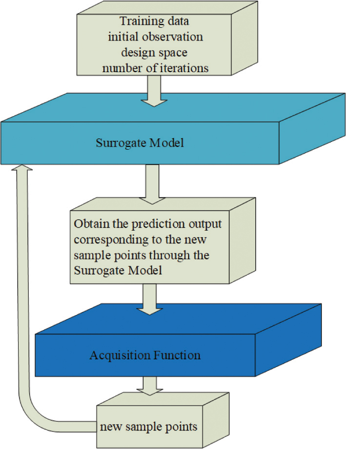
Figure 1: Bayesian optimization framework.
In this paper, the STP is used as the surrogate model of BO, and the kernel function (17) without the property is selected. The hyperparameters of the STP, including the degrees of freedom, noise variance, and hyperparameters of the kernel function, are globally optimized using the pattern search algorithm toolbox [33]. The optimization flowchart is shown in Fig. 2.
| (17) |
The pattern search algorithm uses the negative log-likelihood of STP as the objective function to perform global optimization, obtain the final hyperparameters, and then determine the STP model. The model can output the corresponding prediction function value when given a new observation.
In the BO framework, the acqisition function use the information outputted by the surrogate model to explore the next observation. Common acquisition functions include confidence UCB/LCB [34, 35], EI [36], probability improvement (PI) function [26], entropy search (ES) function [37], EST [38] and ERM [39].
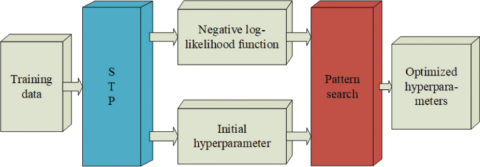
Figure 2: Pattern search toolbox to optimize STP hyperparameters.
Martín presented a detailed derivation of GP upper/lower-confidence bound functions [36]:
| (18) |
| (19) |
Where is the assumed given learning rate, which are different from the LCB function under the GP. In this paper, the in LCB are changed to the prediction mean and prediction variance of STP.
Shah proposes a closed-form solution to the EI function for the STP [21]:
| (20) | ||
where
| (21) |
and are represent the predicted mean and variance of STP, respectively, represent the probability density function and distribution function of T distribution, and define the set of hyperparameters of STP.
The estimation strategy function selects the maximum posterior value in each iteration, which can be expressed as , is the event when the point reaches the maximum value. The EST function can be defined explicitly as:
| (22) |
Obtained by approximation, in this paper, the EST method mentioned in the literature [27] is used to obtain approximately . Unlike wang [27], we replace the predicted mean and predicted standard deviation of STP in the function respectively.
As a result, the pseudocode of the proposed BO algorithm, called BO-STP-EST in the paper, is presented in Algorithm 1.
Algorithm 1 BO-STP-EST.
0: Sample set, ;Initial point,;The number of iterations,iters;Lower bound and upper bound of the design space;
1: for each do
2: → Optimize Hyperparameters for STP using pattern search algorithm, and then train STP;
3: Obtain the posterior prediction mean and posterior variance of by the trained STP;
4: , Get the new sample points by the acquisition function;
5: , Use the trained STP to predict the objective function value corresponding to the input sample point;
6: take the current minimum value, ake the corresponding sample value;
7: end for
4 NUMERICAL EXPERIMENT
In order to verify the generalization performance and global optimization effect of the proposed BO-STP-EST algorithm, numerical experiment is carried out based on the multimodal function (23), where the independent variable interval is [512, 512]. So we finally obtained the training data through the program. The experimental goal is to find the global minimum of this function, and the total number of iterations is set to 50. To verify the performance of the algorithm, we compare it with the BO-GP-LCB [1], BO-GP-EST [27], BO-STP-ERM [23], BO-STP-EI [21], and BO-STP-LCB. For the STP in the models of BO-STP-ERM, BO-STP-LCB, and BO-STP-EI, global optimization is not implemented. The experimental results are shown in Figs. 3 and 4.
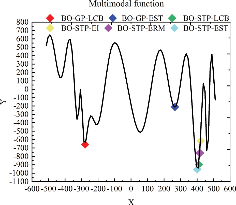
Figure 3: The found minimum value by different models.
| (23) |
It can be seen intuitively from Fig. 3 that only the BO-STP-EST proposed in this paper finds the global minimum of the multimodal function. Models such as BO-GP-LCB and BO-GP-EST are trapped in the local minimum of the function, and other BO algorithms are close to the global minimum of the function, which shows that the proposed BO algorithm has a strong global optimization ability. As can be seen from Fig. 4, since we set the first iteration to be the new sample point explored by the model corresponding to the objective function value, the starting points in the figure are inconsistent, which also just shows that the ability of different models to explore sample points is different.
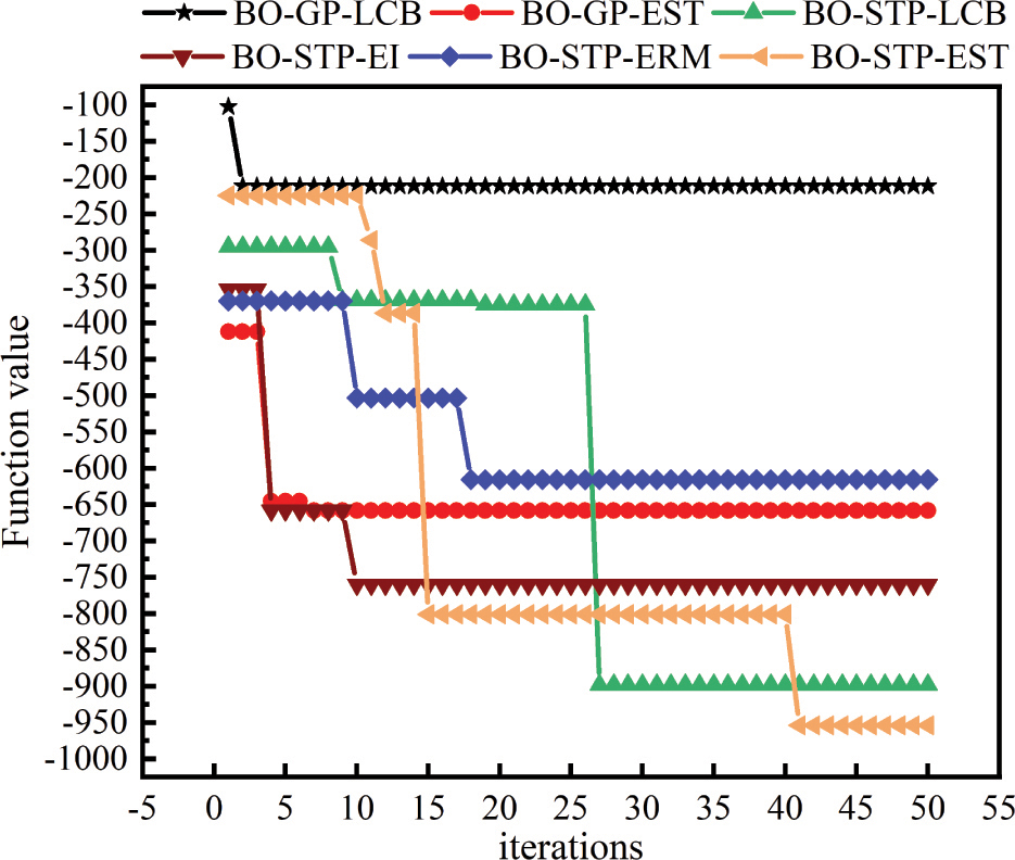
Figure 4: Function value vs. iteration numbers of different models.
Although the objective function value obtained by BO-GP-LCB for the first time is the smallest, it never explores a function value smaller than the current value after 4th time. Compared with the same acquisition function with EST, the exploration ability of the BO algorithm with the GP as the surrogate model is much lower than that of the BO algorithm with the STP as the surrogate model. Compared with the same surrogate model algorithm, the prediction accuracy of the proposed BO-STP-EST algorithm after hyperparameter optimization is significantly higher than that of other models.
5 OPTIMAL DESIGN OF MICROSTRIP ANTENNAS
5.1 Printed dipole antenna
The printed dipole antenna comes from the literature [40] and its structure is shown in Fig. 5. The whole antenna can be divided into five parts, which are the dielectric layer, the dipole antenna arm, the microstrip balun line, the microstrip transmission line, and the antenna feeding surface, The dimensional parameters of the antenna are shown in Table 1. The working frequency of the antenna is 2.25 GHz-2.72 GHz, and the design index include that its working frequency is 2.45 GHz, and the return loss S11 is less than 15 dB.
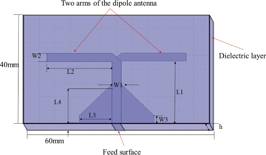
Figure 5: The found minimum value by different models.
As shown in Fig. 5, the antenna has many variables that affect its performance. We select five size variables that have more significant impact as input, as shown in Table 2, including the transmission line length L1, one dipole arm the length L2, the side length L3 of the balun triangle, the right angle length L4 of the base of the balun triangle, and the width W3 of the balun rectangle.
Therefore, the input is , the output is the resonant frequency, while other parameters are fixed. The HFSS-MATLAB-API [41] program is used for the co-simulation of the antenna using the orthogonal experiment method. The frequency sweep range is 2 GHz through 3 GHz, and the step size is 0.01 GHz. So, each group of antenna size variables corresponds to 100 resonance frequency points. The training sample size is .
Table 1: Antenna size parameters
| Variable | Value/mm |
|---|---|
| L1 | 21.5 |
| L2 | 21.5 |
| L3 | 9.8 |
| W1 | 3 |
| W2 | 3 |
| W3 | 3.5 |
| 4.4 | |
| h | 1.6 |
According to the design index of the antenna, the design objective function is (24), where , is the predicted resonant frequency.
Table 2: Design range and initial design value of the printed dipole antenna
| Variable | Min/mm | Max/mm | Initial value/mm |
|---|---|---|---|
| L1 | 21 | 23 | 21.5 |
| L2 | 20 | 22.5 | 21.5 |
| L3 | 9 | 10.5 | 9.8 |
| L4 | 11.5 | 13 | 12.6 |
| W3 | 3 | 5 | 3.5 |
| (24) |
In order to verify the effectiveness of the BO-STP-EST algorithm proposed in this paper, the BO-GP-LCB, BO-GP-EST, BO-STP-LCB, BO-STP-EI, BO-STP-ERM, and the BO-STP-EST are compared. The iterative performance of the objective function under different models, the optimization results of the antenna size and the actual simulation results of the optimized antenna size are verified by experiments. The design space and initial sample points are shown in Table 2, and the total number of iterations is 50 times. The experimental environment is Inter(R)Corte(TM)i5-7500 CPU @ 3.40 GHz 16GB RAM, MATLAB2019b.
Table 3: Optimization results of different models of the printed dipole antenna
| Model | L1 | L2 | L3 | L4 | W3 | Iteration | time | |
| BO-GP-LCB | 23 | 20.1999 | 9.0208 | 12.6053 | 3 | 41 | 1.53e-02 | 106.8259 |
| BO-GP-EST | 22.4373 | 20.7785 | 9 | 12.9988 | 3.2000 | 8 | 8.03e-04 | 105.4107 |
| BO-STP-LCB | 23 | 22.5000 | 10.6000 | 11.5000 | 3 | 20 | 1.55e-02 | 60.3916 |
| BO-STP-EI | 22.8226 | 21.2913 | 9.6366 | 12.1941 | 3.8591 | 5 | 2.65e-04 | 115.4727 |
| BO-STP-ERM | 22.4044 | 20.0226 | 9.9722 | 11.5997 | 4.5191 | 19 | 8.60e-05 | 137.3362 |
| BO-STP-EST | 23 | 21.0537 | 10.5999 | 11.5000 | 3 | 3 | 2.88e-05 | 93.5832 |
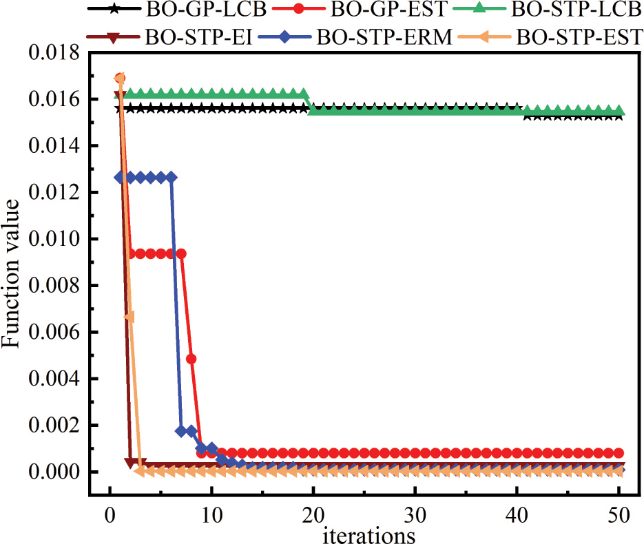
Figure 6: The found minimum value by different models.
From Fig. 6 and Table 3, we can see that the proposed BO-STP-EST exhibits a good generalization ability, and it can find the minimum in a few iterations. Compared with the BO algorithm with GP as the surrogate model, BO-GP-LCB find a smaller value in the 41st time, but this minimum value is very different from other models. For the same acquisition function, BO-GP-EST takes more time to find the minimum at the 8th iteration, and the proposed BO-STP-EST performs much better than BO-GP-EST, where it finds the minimum value at the 3rd iteration. Compared with other models with STP, BO-STP-EI and BO-STP-ERM are not as good as BO-STP-EST in terms of the objective function and time consumption because the optimized STP has fitting higher-degree posterior outputs which makes the EST collection function have stronger exploration ability.
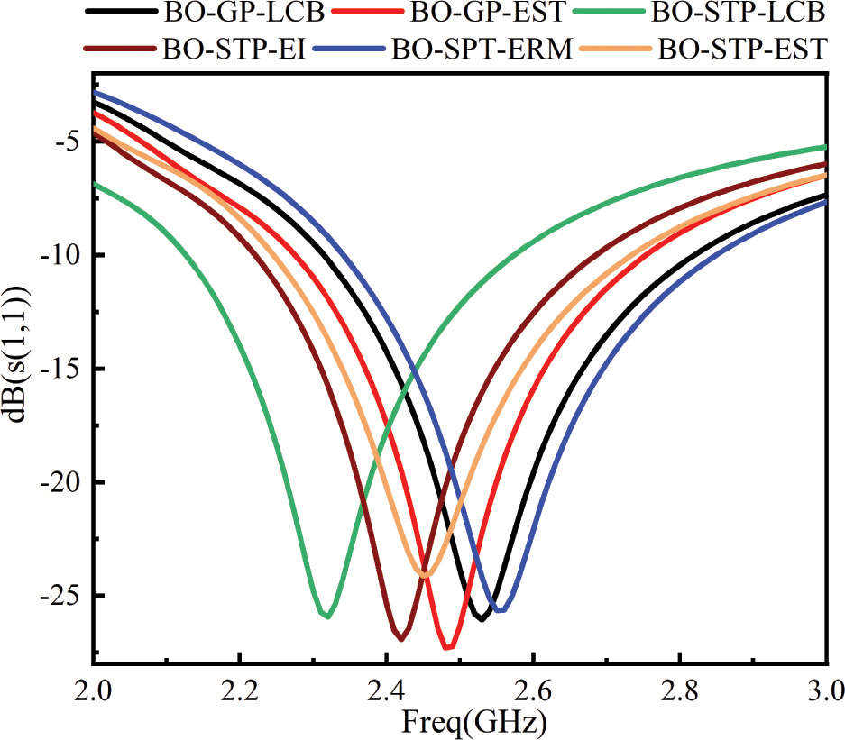
Figure 7: The found minimum value by different models.
The antenna optimization results in Fig. 7 verified by HFSS illustrate that, for the design index of the resonant frequency of the antenna, only the proposed BO-STP-EST achieves the design targets with the resonant frequency 2.45 GHz and where . The resonant frequency points predicted by other models have certain errors, which are also in line with the prediction results of the objective function in Table 3 and Table 4. It can be concluded from the above tables and figures that the proposed BO-STP-EST has greater advantages in convergent speed and accuracy than other models.
Table 4: The actual resonant frequencies optimized by different models of the printed dipole antenna
| Model | Resonant frequency/GHz | Return loss/dB |
|---|---|---|
| BO-GP-LCB | 2.53 | 26.0488 |
| BO-GP-EST | 2.49 | 27.2250 |
| BO-STP-LCB | 2.32 | 25.9310 |
| BO-STP-EI | 2.42 | 26.9227 |
| BO-STP-ERM | 2.56 | 25.6303 |
| BO-STP-EST | 2.45 | 24.1248 |
5.2 E-shaped antenna
Table 5: Design range and initial design value of the E-shape antenna
| Variable | Min/mm | Max/mm | Initial value/mm |
|---|---|---|---|
| L | 25 | 35 | 26 |
| W | 20 | 28 | 29 |
| ls | 2 | 8 | 4 |
| ws | 4 | 18 | 7 |
| h | 1.57 | 3.57 | 1.6 |
Table 6: Results obtained by different models for the E-shape antenna
| Model | L | W | ls | ws | h | Iteration | time | |
| BO-GP-LCB | 35 | 28 | 2 | 4.84 | 3.57 | 6 | 0.105 | 106.83 |
| BO-GP-EST | 30.09 | 24.12 | 5 | 14.5 | 2.57 | 12 | 1.616e-05 | 115.19 |
| BO-STP-LCB | 25 | 28 | 2 | 18 | 1.64 | 28 | 0.0424 | 165.4 |
| BO-STP-EI | 30.89 | 20.30 | 2.50 | 16.05 | 2.77 | 41 | 0.0372 | 198.42 |
| BO-STP-ERM | 26.20 | 27.71 | 8 | 16.10 | 2.62 | 42 | 7.626e-05 | 220 |
| BO-STP-EST | 35 | 28 | 8 | 4.95 | 3.57 | 7 | 5.313e-05 | 197.03 |
The E-shaped antenna is evolved from the rectangular patch antenna, and two identical parallel slot antennas are formed by using the slot-loading method [42]. For the E-shaped antenna, it is easy to obtain good performance by adjusting the shape of the slot, which is very suitable for use in portable communication and miniaturized equipment. The E-shaped antenna is shown in Fig. 8, which consists of a radiation patch, a ground plate, a dielectric plate, and a feeding point.
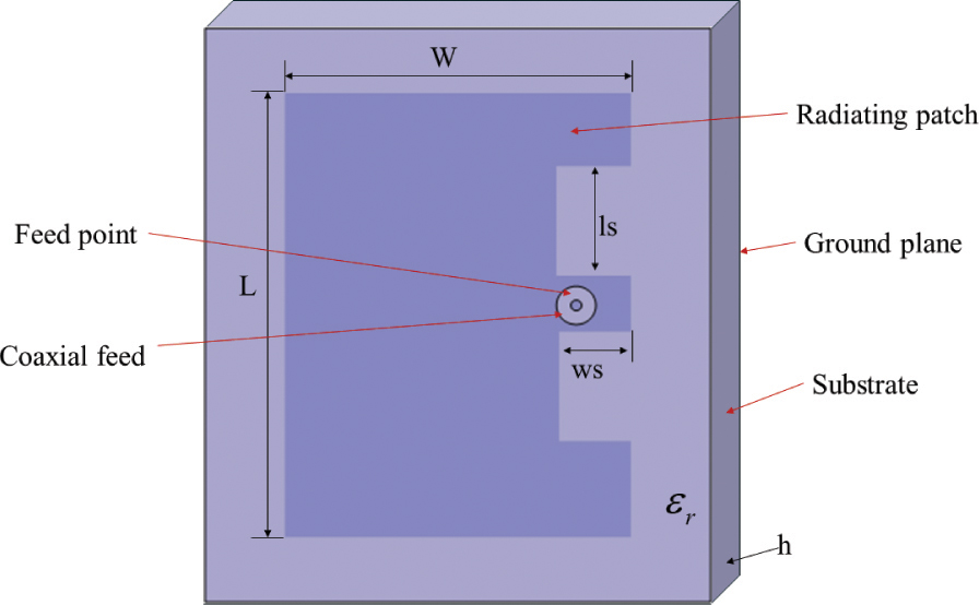
Figure 8: E-shaped antenna structure diagram.
The design index is the working frequency 3.50 GHz, where the return loss S11 is less than 10 dB. According to the structure of the antenna, several parameters that greatly affect the performance of the antenna, including , are selected as the training input of the model, and the rests are unchanged, including the dielectric material , as shown in Table 5.
Therefore, the input is , and the output is . The frequency sweep range is 2 GHz-5 GHz, the step size is 0.01 GHz. So, each group of antenna size variables corresponds to 100 resonance frequency points, and the training data is finally obtained.
To verify the generalization and optimization performance of the proposed BO-STP-EST, we compare the performances of the BO-GP-LCB, BO-GP-EST, BO-STP-LCB, BO-STP-EI, and BO-STP-ERM. The design objective function is (25), where , is the predicted resonant frequency.
| (25) |
The experiment compares the differences in the number of iterations, the minimum value, and the duration of the six models. The results are shown in Table 6. The return loss of the antenna obtained by the final optimization of each model is also compared, and the results are shown in Fig. 9 and Table 6.
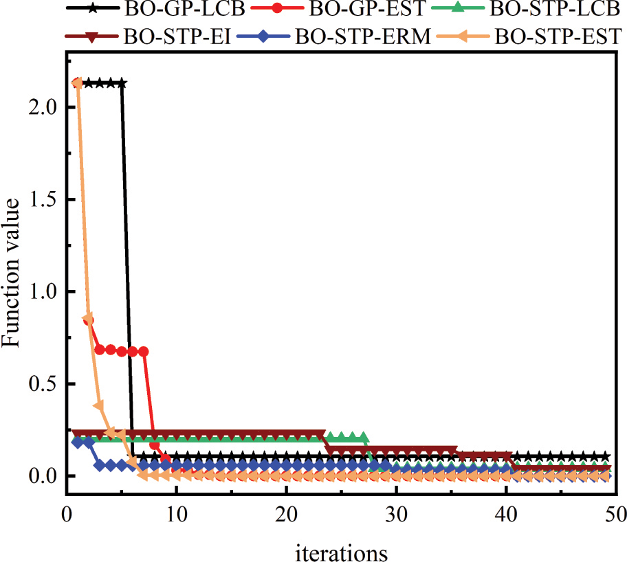
Figure 9: Objective functions vs. iteration of different model for the E-shape antenna.
As can be seen from Fig. 9, since the sample points recorded in the first setting of the model program are ones collected by the acquisition function, we can see the ability of different models to explore the sample points in the sample space. Compared with the same acquisition function EST, although the value of the objective function corresponding to the sample points first explored by the proposed BO-STP-EST algorithm is greater than BO-GP-EST, it is much stronger than BO-GP-EST in the subsequent exploration ability. It finds the global minimum value in the 7th iteration and is better than that found by BO-GP-EST in the 12th iteration.
Compared with other models by STP, BO-STP-EST can find the minimum value of objective function which is much smaller than BO-STP-LCB and BO-STP-EI. As we can see from table 6,7, although the final objective function value found by BO-STP-ERM is close to BO-STP-EST, it takes more time. Therefore, BO-STP-EST is still the most competitive among several models in terms of minimum value and time-consuming of objective function.
Table 7: The actual resonant frequencies optimized by different models of the printed dipole antenna
| Model | Resonant frequency/GHz | Return loss/dB |
|---|---|---|
| BO-GP-LCB | 3.49 | 13.460 |
| BO-GP-EST | 3.69 | 33.945 |
| BO-STP-LCB | 3.30 | 17.399 |
| BO-STP-EI | 4.27 | 20.067 |
| BO-STP-ERM | 3.19 | 28.231 |
| BO-STP-EST | 3.50 | 12.837 |
In the experiment of this part, we deliberately reduce the number of training samples, so as to verify that the hyperparametric optimization of the model can improve the prediction ability of the algorithm proposed in this paper when the training samples are reduced. The simulation results (Fig. 10) verified by HFSS show that when the training samples are reduced (Table 7), the prediction accuracy of the different models mentioned in the paper begins to decline, however, the accuracy of the BO-STP-EST is much higher than that of the algorithm without global hyperparametric optimization. Taking the STP as surrogate model, the algorithm still maintains good prediction accuracy under the condition of reducing the number of training samples. At the same time, the proposed BO-STP-EST realizes the design index of at the resonant frequency at 3.5 GHz. It shows that the hyper-parameter optimization of surrogate model can improve the accuracy and optimization performance of Bayesian optimization algorithm.
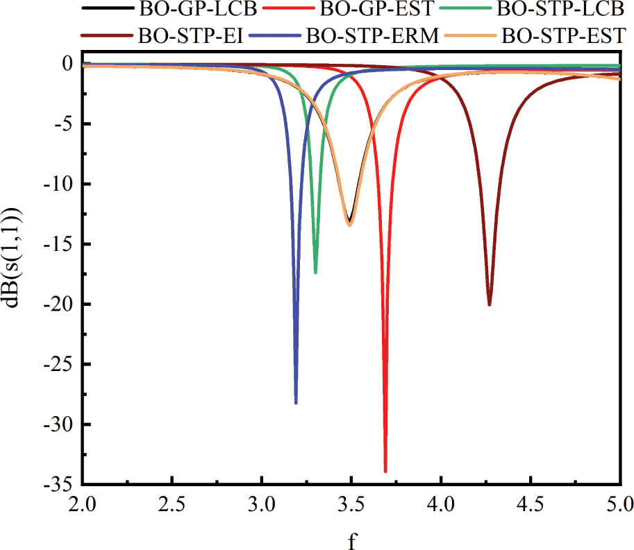
Figure 10: Simulation results obtained by different models for the E-shape antenna.
6 CONCLUSION
This paper proposes a BO algorithm that combines an improved maximum evaluation policy function with a hyperparameter-optimized STP. Numerical experimental verification of finding the minimum value through multimodal functions shows that the proposed BO algorithm with the STP as the surrogate model has better prediction accuracy than these with the GP as the surrogate model. At the same time, the acquisition function EST can improve the exploration ability of the BO algorithm. The proposed algorithm in this paper is applied to the antenna modeling problems, and the design index can be well completed. The simulation results of electromagnetic simulation software also verify the effectiveness of the algorithm.
Although the proposed algorithm is only applied to the optimization problem of single-band antennas in this paper, following, we will study the multi-band antenna optimization by the proposed algorithm.
ACKNOWLEDGMENT
This work was supported by the special projects in key fields of Guangdong Universities of China under No. 2022ZDZX1020, the scientific research capacity improvement project of key developing disciplines in Guangdong Province of China under No. 2021ZDJS057, and the university scientific research project of Bureau of Education of Guangzhou Municipality of China under No. 202234598.
REFERENCES
[1] L. Acerbi and W. J. Ma, “Practical Bayesian optimization for model fitting with Bayesian adaptive direct search,” Advances in Neural Information Processing Systems, vol. 30, 2017.
[2] V. Nguyen, S. Schulze, and M. Osborne, “Bayesian optimization for iterative learning,” Advances in Neural Information Processing Systems, vol. 33, pp. 9361-9371, 2020.
[3] M. Wistuba and J. Grabocka, “Few-shot bayesian optimization with deep kernel surrogates,” arXiv preprint arXiv:2101.07667, 2021.
[4] D. Yenicelik, “Parameter Optimization using high-dimensional Bayesian Optimization,” arXiv preprint arXiv:2010.03955, 2020.
[5] J. Mockus, V. Tiesis, and A. Zilinskas, “The application of Bayesian methods for seeking the extremum,” Towards Global Optimization, vol. 2, no. 117-129, p. 2, 1978.
[6] L. Breiman, “Random forests,” Machine Learning, vol. 45, no. 1, pp. 5-32, 2001.
[7] J. Snoek, O. Rippel, K. Swersky, R. Kiros, N. Satish, N. Sundaram, M. Patwary, M. Prabhat, and R. Adams, “Scalable bayesian optimization using deep neural networks,” International Conference on Machine Learning, pp. 2171-2180,2015.
[8] S. R. Chowdhury and A. Gopalan, “No-regret algorithms for multi-task bayesian optimization,” International Conference on Artificial Intelligence and Statistics, pp. 1873-1881, 2021.
[9] D. Ginsbourger, R. L. Riche, and L. Carraro, “Kriging is well-suited to parallelize optimization,” Computational Intelligence in Expensive Optimization Problems, pp. 131-162, 2010.
[10] Z. Feng, Q. Zhang, Q. Zhang, Q. Tang, T. Yang, and Y. Ma, “A multiobjective optimization based framework to balance the global exploration and local exploitation in expensive optimization,” Journal of Global Optimization, vol. 61, no. 4, pp. 677-694, 2015.
[11] S. Han, Y. Tian, W. Ding, and P. Li, “Resonant frequency modeling of microstrip antenna based on deep kernel learning,” IEEE Access, vol. 9, pp. 39067-39076, 2021.
[12] T. Zhang, Y. Tian, X. Chen, and J. Gao, “Antenna Resonant Frequency Modeling based on AdaBoost Gaussian Process Ensemble,” Applied Computational Electromagnetics Society (ACES) Journal, pp. 1485-1492, 2020.
[13] A. O’Hagan, “On outlier rejection phenomena in Bayes inference,” Journal of the Royal Statistical Society: Series B (Methodological), vol. 41, no. 3, pp. 358-367, 1979.
[14] A. Shah, A. Wilson, and Z. Ghahramani, “Student-T processes as alternatives to Gaussian processes,” Artificial Intelligence and Statistics, pp. 877-885, 2014.
[15] A. Solin and S. Särkkä, “State space methods for efficient inference in Student-t process regression,” Artificial Intelligence and Statistics, pp. 885-893, 2015.
[16] Q. Tang, L. Niu, Y. Wang, T. Dai, W. An, J. Cai, and S.-T. Xia, “Student-T process regression with Student-T likelihood,” IJCAI, pp. 2822-2828, 2017.
[17] Z. Chen, B. Wang, and A. N. Gorban, “Multivariate Gaussian and Student-T process regression for multi-output prediction,” Neural Computing and Applications, vol. 32, no. 8, pp. 3005-3028,2020.
[18] W. Wang, Q. Yu, and M. Fasli, “Altering Gaussian process to Student-T process for maximum distribution construction,” International Journal of Systems Science, vol. 52, no. 4, pp. 727-755, 2021.
[19] L. Kang, R.-S. Chen, N. Xiong, Y.-C. Chen, Y.-X. Hu, and C.-M. Chen, “Selecting hyper-parameters of Gaussian process regression based on non-inertial particle swarm optimization in Internet of Things,” IEEE Access, vol. 7, pp. 59504-59513, 2019.
[20] Z. Le, L. Zhong, Z. Jianqiang, and R. Xiongwei, “Improved Gaussian process model based on artificial bee colony algorithm optimization,” Journal of National University of Defense Science and Technology, p. 7, 2014.
[21] A. Shah, A. G. Wilson, and Z. Ghahramani, “Bayesian optimization using Student-T processes,” NIPS Workshop on Bayesian Optimization, 2013.
[22] B. D. Tracey and D. Wolpert, “Upgrading from Gaussian processes to Student’s T processes,” 2018 AIAA Non-Deterministic Approaches Conference, p. 1659, 2018.
[23] C. Clare, G. Hawe, and S. McClean, “Expected regret minimization for bayesian optimization with Student’s-T processes,” Artificial Intelligence and Pattern Recognition, pp. 8-12, 2020.
[24] W. Ding, Y. Tian, P. Li, H. Yuan, and R. Li, “Antenna optimization based on master-apprentice broad learning system,” International Journal of Machine Learning and Cybernetics, vol. 13, no. 2, pp. 461-470, 2022.
[25] J. Gao, Y. Tian, X. Zheng, and X. Chen, “Resonant frequency modeling of microwave antennas using Gaussian process based on semisupervised learning,” Complexity, vol. 2020, 2020.
[26] H. M. Torun, M. Swaminathan, A. K. Davis, and M. L. F. Bellaredj, “A global Bayesian optimization algorithm and its application to integrated system design,” IEEE Transactions on Very Large Scale Integration (VLSI) Systems, vol. 26, no. 4, pp. 792-802, 2018.
[27] Z. Wang, B. Zhou, and S. Jegelka, “Optimization as estimation with Gaussian processes in bandit settings,” Artificial Intelligence and Statistics, pp. 1022-1031, 2016.
[28] C. E. Rasmussen, “Gaussian processes in machine learning,” Summer School on Machine Learning, pp. 63-71, 2003.
[29] W. P. du Plessis and J. P. Jacobs, “Improved Gaussian Process Modelling of On-Axis and Off-Axis Monostatic RCS Magnitude Responses of Shoulder-Launched Missiles,” Applied Computational Electromagnetics Society (ACES) Journal, pp. 1750-1756, 2019.
[30] J. Vanhatalo, P. Jylänki, and A. Vehtari, “Gaussian process regression with Student-t likelihood,” Advances in Neural Information Processing Systems, vol. 22, 2009.
[31] Q. T. Y. Wang and S.-T. Xia, “Student-T process regression with dependent Student-t noise,” ECAI 2016: 22nd European Conference on Artificial Intelligence, 29 August-2 September 2016, The Hague, The Netherlands-Including Prestigious Applications of Artificial Intelligence (PAIS 2016), vol. 285, p. 82, 2016.
[32] S. Greenhill, S. Rana, S. Gupta, P. Vellanki, and S. Venkatesh, “Bayesian optimization for adaptive experimental design: A review,” IEEE Access, vol. 8, pp. 13937-13948, 2020.
[33] A. M. Beigi and A. Maroosi, “Parameter identification for solar cells and module using a hybrid firefly and pattern search algorithms,” Solar Energy, vol. 171, pp. 435-446, 2018.
[34] D. Calandriello, L. Carratino, A. Lazaric, M. Valko, and L. Rosasco, “Gaussian process optimization with adaptive sketching: Scalable and no regret,” Conference on Learning Theory, pp. 533-557, 2019.
[35] L. A. Martín and E. C. Garrido-Merchán, “Many Objective Bayesian Optimization,” arXiv preprint arXiv:2107.04126, 2021.
[36] L. Tani and C. Veelken, “Comparison of Bayesian and particle swarm algorithms for hyperparameter optimisation in machine learning applications in high energy physics,” arXiv preprint arXiv:2201.06809, 2022.
[37] J. M. Hernández-Lobato, M. W. Hoffman, and Z. Ghahramani, “Predictive entropy search for efficient global optimization of black-box functions,” Advances in Neural Information Processing Systems, vol. 27, 2014.
[38] I. Bogunovic and A. Krause, “Misspecified gaussian process bandit optimization,” Advances in Neural Information Processing Systems, vol. 34, 2021.
[39] V. Nguyen and M. A. Osborne, “Knowing the what but not the where in Bayesian optimization,” International Conference on Machine Learning, pp. 7317-7326, 2020.
[40] W.-T. Ding, F. Meng, Y.-B. Tian, and H.-N. Yuan, “Antenna optimization based on auto-context broad learning system,” International Journal of Antennas and Propagation, vol. 2022, 2022.
[41] W. Tian, D. Wu, Q. Chao, Z. Chen, and Y. Wang, “Application of genetic algorithm in M N reconfigurable antenna array based on RF MEMS switches,” Modern Physics Letters B, vol. 32, no. 30, p. 1850365, 2018.
[42] D. Ustun, A. Toktas, and A. Akdagli, “Deep neural network–based soft computing the resonant frequency of E–shaped patch antennas,” AEU-International Journal of Electronics and Communications, vol. 102, pp. 54-61, 2019.
BIOGRAPHIES

Qing Li was Born in Anqing, Anhui Province, China, studying in Jiangsu University of science and technology, master’s degree, research direction: intelligent optimization algorithm, intelligent electromagnetic optimization.

Fei Meng was born in Shenyang, Liaoning Province, China, in 1977. She is currently with the School of Information and Communication Engineering, Guangzhou Maritime University, Guangzhou, China. She has authored and coauthored 10 Journal papers. Her research interest is surrogates and their applications.

Yubo Tian was born in Tieling, Liaoning Province, China, in 1971. He received the Ph.D. degree in radio physics from the De-partment of Electronic Science and Engineering, Nanjing University, Nanjing, China. He has been a visiting scholar at the University of California Los Angeles in 2009 and the Griffith University in 2015, respectively. From 1997 to 2004, he was with the Department of Information Engineering, Shenyang University, Shenyang, China. From 2005 to 2020, he was with the School of Electronics and Information, Jiangsu University of Science and Technology, Zhenjiang, China, where he was a full professor and vice Dean from 2011. He is currently with the School of Information and Communication Engineering, Guangzhou Maritime University, Guangzhou, China. Dr. Tian has authored and coauthored more than 100 Journal papers and 3 books. He also holds more than 20 filed/granted China patents. His current research interest is Machine Learning methods and their applications in electronics and electromagnetics.

Xiaoyan Wang studying in Jiangsu University of science and technology, master’s degree, research direction: intelligent optimization algorithm, intelligent electromagnetic optimization.
ACES JOURNAL, Vol. 37, No. 8, 856–866.
doi: 10.13052/2022.ACES.J.370804
© 2022 River Publishers