Obtaining Feasible Minimum Side Lobe Level for Narrow Beam Width Using Convex Optimization in Linear, Planar, and Random Antenna Arrays
Rana R. Shaker and Jafar R. Mohammed
Department of Communication Engineering, College of Electronic Engineering, Ninevah University, Mosul-41002, Iraq
rana.raad2021@stu.uoninevah.edu.iq; jafar.mohammed@uoninevah.edu.iq
Submitted On: April 30, 2022; Accepted On: October 6, 2022
Abstract
In many applications, the radiating elements of the used antenna may be configured in the form of a one-dimensional linear array, or two-dimensional planar array or even random array. In such applications, a simple optimization algorithm is highly needed to optimally determine the excitation amplitudes and phases of the array elements to maximize the system’s performance. This paper uses a convex optimization instead of other complex global stochastic optimizations to synthesize a linear, planar, and random array patterns under pre-specified constraint conditions. These constraints could be either fixed beam width with the lowest possible sidelobe levels or fixed sidelobe level with narrower possible beam width. Two approaches for array pattern optimization have been considered. The first one deals with the problem of obtaining a feasible minimum sidelobe level for a given beam width, while the second one tries to obtain a feasible minimum beam width pattern for a given sidelobe level. Both optimization approaches were applied to the linear, planar, and random arrays. Simulation results verified the effectiveness of both optimization approaches and for all considered array configurations.
Index Terms: beam width minimization, convex optimization, linear array, planar array, random array, sidelobe level minimization.
1 INTRODUCTION
In most antenna array applications, low sidelobe levels with narrow beam width patterns (i.e., maximum directivities) are critical to minimize the undesirable effects of the interfering and noise signals that may cause false target indications and degrade the overall system performance. Generally, the radiating elements of the antenna arrays can be arranged as a one-dimensional linear array, two-dimensional planar array, or even random array configurations. In the linear and planar arrays, the inter-element spacing is usually regular and uniform, while in the random arrays they are irregular and non-uniform. Unlike the linear arrays where their radiation patterns can be scanned either on the azimuth or elevation angles, the radiation patterns of the planar arrays can be simultaneously scanned to any angle in the azimuth and elevation planes. Thus, planar arrays are most widely used in practice due to their advantages and versatility [1].
The regularly spaced and uniformly excited linear and planar arrays have many good radiation characteristics such as narrow beam width, good directivity, and simple excitation weight vector, but they suffer from high sidelobe levels (SLLs) which are about 13.2 dB. Such high SLLs may cause many problems with false target indications. Usually, the beamwidth, sidelobe level, and many other array pattern characteristics can be controlled by adjusting one or more of the following array design parameters; geometrical layout of the array elements, the excitation phases, and amplitudes of the array elements, inter-element spacing, and the elementary pattern of each element [2]. In this work, the excitation amplitudes and phases were used to design the linear and the planar arrays. Whereas in the random arrays, first the inter-element spacing is determined randomly, then, the excitation amplitudes and phases of the random elements were optimized to get the required array pattern.
In the literature, many researchers have studied these design parameters and found that the SLL can be reduced by tapering the excitation amplitudes of the array elements. Therefore, many tapers based on deterministic approaches have been suggested such as Dolph, Taylor, triangular, and raised cosine, to name just a few [2, 3]. Specifically, the Dolph-Tschebyscheff approach suggested a certain distribution for the element excitations such that the corresponding array pattern has a minimum widening factor in the beam width for a given sidelobe level. In other words, as the beam width decreases, the side lobe level increases and vice versa. Although these tapering methods successfully reduced the sidelobe levels, these good results came at the cost of widening the beam width. Thus, there was always a trade-off between the required sidelobe level and the desired beam width pattern [4].
In an attempt to maintain the beam width unchanged while reducing the sidelobe levels, several simple analytical and numerical methods were presented in [5, 6, 7] where the excitation amplitudes and phases of just two side elements in the linear array were controlled. Then, the method was further extended to the planar arrays where the excitation amplitudes and phases of the boundary elements were modified to achieve the required radiation pattern [8].
On the other hand, many optimization techniques such as genetic algorithm [9], particle swarm optimization [10], simulated annealing [11], differential evolution algorithm [12], and others [13] have been also used for array synthesis. However, the computational complexity of these globally optimized methods is high, especially when dealing with relatively large arrays.
Interestingly, the problem of the array synthesis with a feasible minimum sidelobe level for a given beam width or vice versa can be successfully solved by using convex optimization methods. First, by converting the problem into convex, then the optimal solution becomes much easier and faster than that of other global optimization methods. In fact, many array synthesis scenarios are convex in nature and they can be simply solved without recalling other complex optimization methods such as genetic algorithms [14, 15] or Modified Seagull optimization [16, 17].
In this paper, the convex optimization [18] was applied to the linear, planar, and random arrays to obtain the desired radiation patterns where the excitation amplitude and phase of the individual array elements are optimized. To proceed with the optimization process, two constraint strategies were suggested. The first one includes the finding of the feasible minimum sidelobe level for a given beam width pattern, while the other one includes the finding of the feasible minimum beam width pattern for a given sidelobe level. The effectiveness of both strategies in designing linear, planar, and random arrays was fully illustrated and verified.
2 THE CONVEX OPTIMIZED METHOD
A regularly spaced two-dimensional rectangular planar array composed of N rows and M columns of isotropic radiating elements are considered. The elements are distributed uniformly on the xy plane with separation distances and in the x and y directions, respectively. For uniformly spaced linear arrays, the array size will be either or according to the considered axis. In general, the array factor of two-dimensional elements can be given by:
| (1) |
where is the wavelength at the operating frequency, and are the elevation and azimuth angles, respectively, and , are the progressive phase shifts in the x and y directions, respectively. and are the steered angles. Finally, represents the amplitude and phase excitations of the (n,m) element.
For random arrays, the elements are randomly located along the x and y-axes and the inter-element spacing is irregular. Thus, (1) can be rewritten as:
| (2) |
where and are the random locations of the (n,m) element. From (1) and (2), it is clear that the total number of adjustable excitation elements, , is which is quite large, especially for large arrays. Thus, the uses of global stochastic optimizations such as genetic algorithms are associated with high complexity and slow convergence. Further, in many cases, the optimal solution may not require such a highly complex-global optimization algorithm since the searching space may be convex. Therefore, such problem can be solved efficiently by the convex optimization where the unknown array excitations, , constitutes a set of linear functions on a convex space.
The convex optimization problem is formulated as the determination of the excitation amplitudes and phases of the array elements such that the resulting radiation pattern satisfies one of the following two cases.
Case 1: Obtaining feasible minimum sidelobe level for a given beam width
In this case, the convex optimization minimizes the sidelobe level outside the beamwidth of the array pattern and it has unit sensitivity at the target direction to avoid any distortion in the main beam peak. These constraints are written as follows:
| (3) |
Subject to:
| (4) |
| (5) |
where is the feasible starting value of the sidelobe level in the elevation plane for a fixed value of azimuth angle, and is the required first null to null beam width in the elevation plane. The constraint in (4) aims at preserving the unit gain in the target direction, while the constraint in (2) is for obtaining the feasible minimum sidelobe level for a given beam width pattern.
Case 2: Obtaining minimum beam width pattern for a given sidelobe level
In this case, the optimized array pattern is designed such that it has unit sensitivity at the desired target direction, satisfies the constraint on the sidelobe level outside the main beam, and minimizes the beamwidth of the array pattern. The results of applying these two cases are shown in the following section.
3 SIMULATION RESULTS
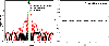
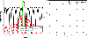
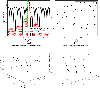
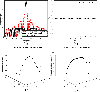
In this section, many examples are presented and investigated by means of computer simulations to assess the performance of the described optimization methods. Matlab software has been used to obtain the results. In the first example, a uniformly spaced linear array with a total number of elements equal to 36 (i.e., N=36 and M=1) spaced by is considered. The required first null to null beam width (FNBW) of the optimized array pattern was chosen to be equal to that of the standard uniformly excited linear array with 36 elements which is 5, (. Note that the FNBW of the optimized array is restricted to be as narrow as that of the standard uniformly excited linear array while solving for the feasible minimum sidelobe level. The target direction is assumed to be known and equals 0. In this case, the excitation amplitudes and phases are optimized such that the corresponding array factor complies with the imposed constraints according to (3), (4), and (2). Figure 1 shows the radiation pattern of the optimized linear array and its element locations. For comparison purposes, the radiation pattern of the standard uniformly excited linear array is also shown in this figure. From this figure, it is found that the FNBW of the optimized array is exactly equal to that of the standard uniformly excited linear array, and the feasible minimum sidelobe level was 31.8 dB which is much lower than that of the standard uniformly excited linear array, 13.2 dB. The optimized excitation amplitudes and phases are shown in Fig. 2.
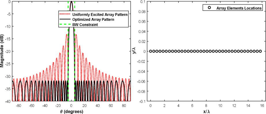
Figure 1: Optimized pattern of the linear array with 361 elements for =5 (left) and its element locations (right).
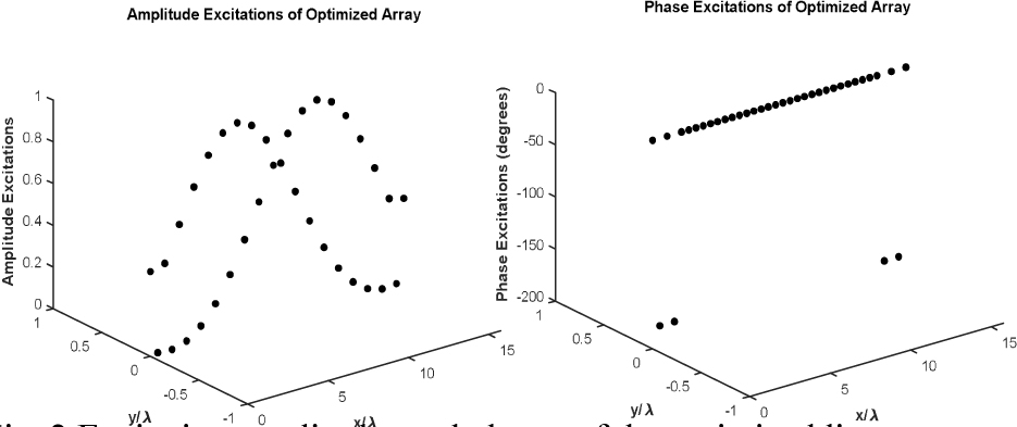
Figure 2: Excitation amplitudes and phases of the optimized linear array whose pattern is shown in Fig. 1.
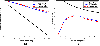
In the second example, a uniformly spaced planar array with elements is considered. Note that the total number of the array elements in all array configurations (linear, planar, and random) was fixed to 36 elements. Again, the same optimization constraints as in the previous example were imposed to obtain the feasible minimum sidelobe level for a given narrow beam width, . The pattern of the optimized planar array and its element locations are shown in Fig. 3, whereas the excitation amplitudes and phases are shown in Fig. 4. In this case, the feasible minimum SLL was 8 dB which is higher than that of the standard uniformly excited linear array, 13.2 dB. Nevertheless, much lower SLL can be obtained for larger values of beam widths.
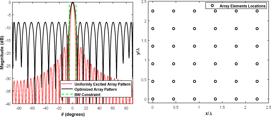
Figure 3: Optimized pattern of the planar array with 66 elements for (left) and its element locations (right).
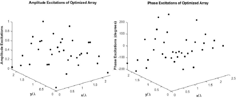
Figure 4: Excitation amplitudes and phases of the optimized planar array whose radiation pattern is shown in Fig. 3.
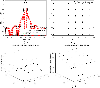
In the third example, a randomly spaced planar array with elements is considered. Again, the beam width constraint was as in the previous examples. The results for the optimized random array are shown in Fig. 5. From this figure, it can be seen that the feasible minimum sidelobe level was 7.7 dB which is also higher than that of the standard uniformly excited linear array, 13.2 dB. Nevertheless, much lower SLL can be obtained for wider beam width as shown in Fig. 6 (a) where the beam width was varied from to and the corresponding feasible minimum SLL was recorded. For these values of beam widths, the directivities of the three array configurations were also plotted as shown in Fig. 6 (b). From these two figures, it can be seen that the linear array gives the feasible minimum SLL and higher directivity. This is mainly because the linear array configuration has wider space diversity than the planar and random arrays, thus, narrower beam width and better directivity can be achieved. Moreover, the feasible minimum SLL can be significantly reduced with an increase in the given
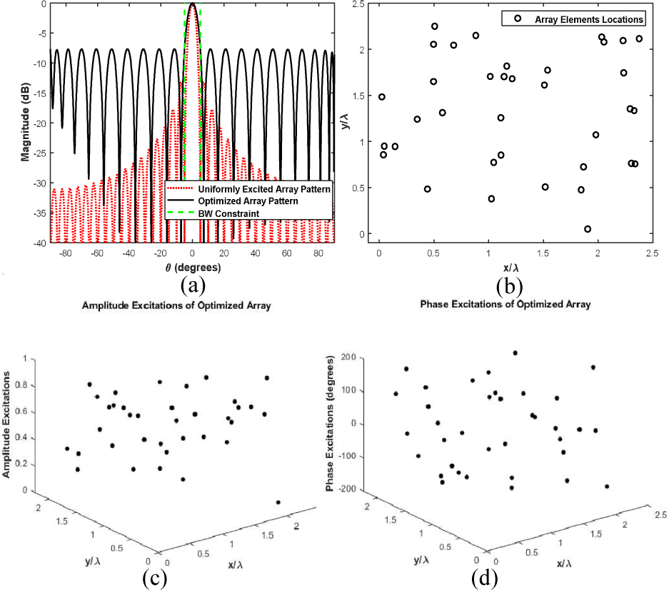
Figure 5: (a) Optimized pattern of the random array with 66 elements for , (b) its element locations, (c) excitation amplitudes, and (d) phases.
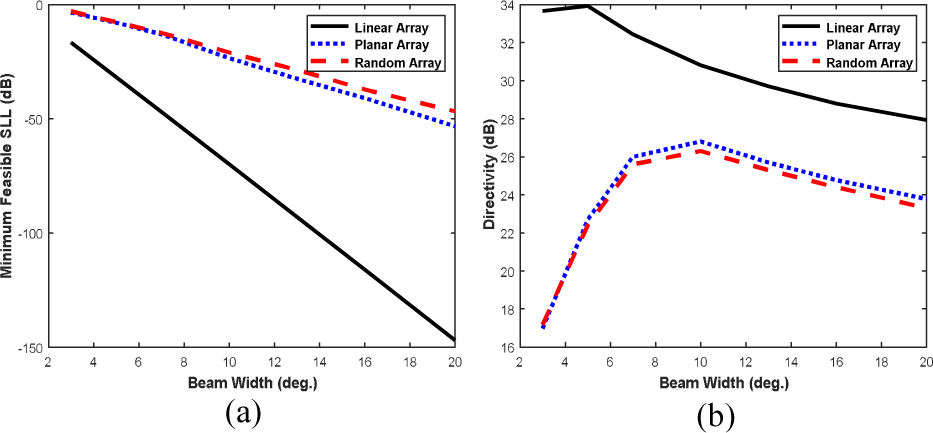
Figure 6: (a) Variation of minimum SLL and (b) directivity.
In the next example, a feasible minimum beam width pattern for a given SLL is investigated where the SLL was fixed at 30 dB, and a feasible minimum beam width for linear, planar, and random arrays was computed as shown in Fig. 7 to Fig. 9. From these figures, it can be seen that the feasible minimum beam width for linear, planar, and random arrays was , , and respectively for given SLL = 30 dB.
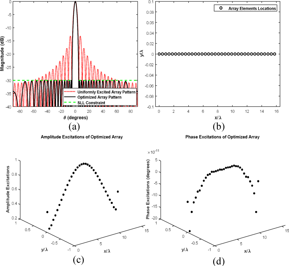
Figure 7: (a) Optimized pattern of the linear array with 361 elements for SLL = 30 dB, (b) its element locations, (c) excitation amplitudes, and (d) phases.
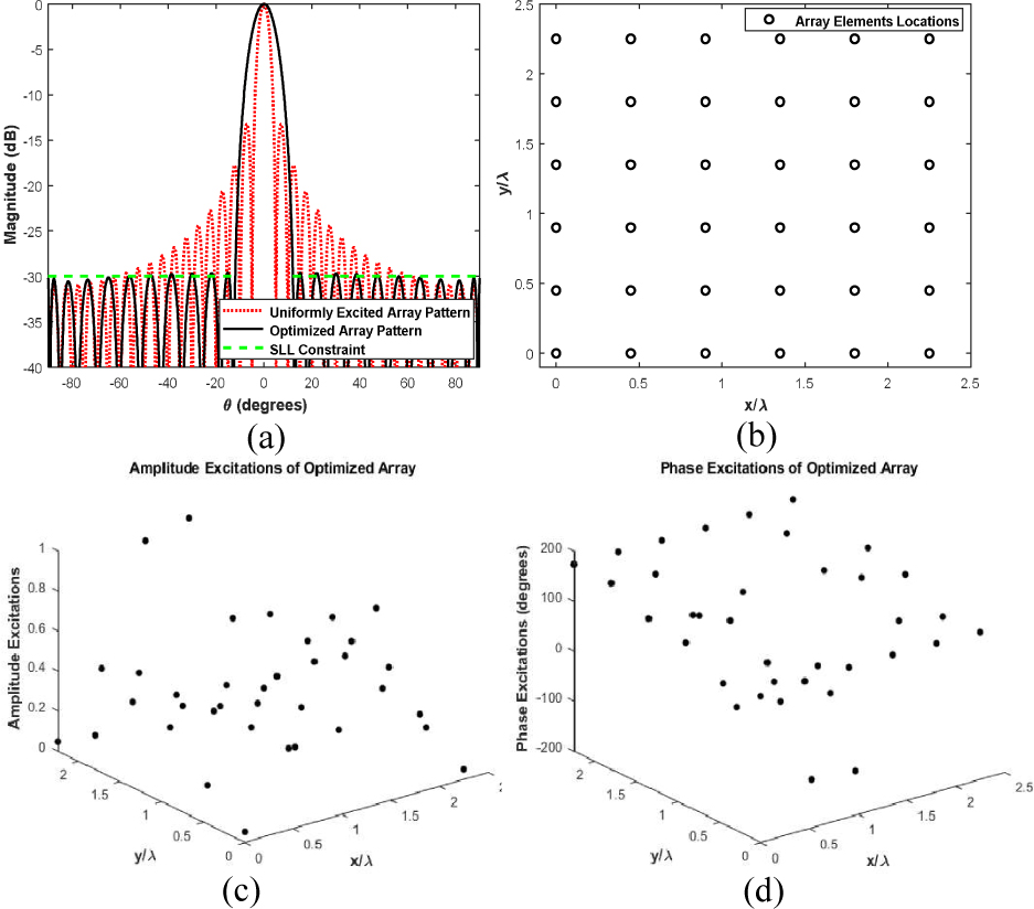
Figure 8: (a) Optimized pattern of the linear array with 66 elements for SLL = 30 dB, (b) its element locations, (c) excitation amplitudes, and (d) phases.
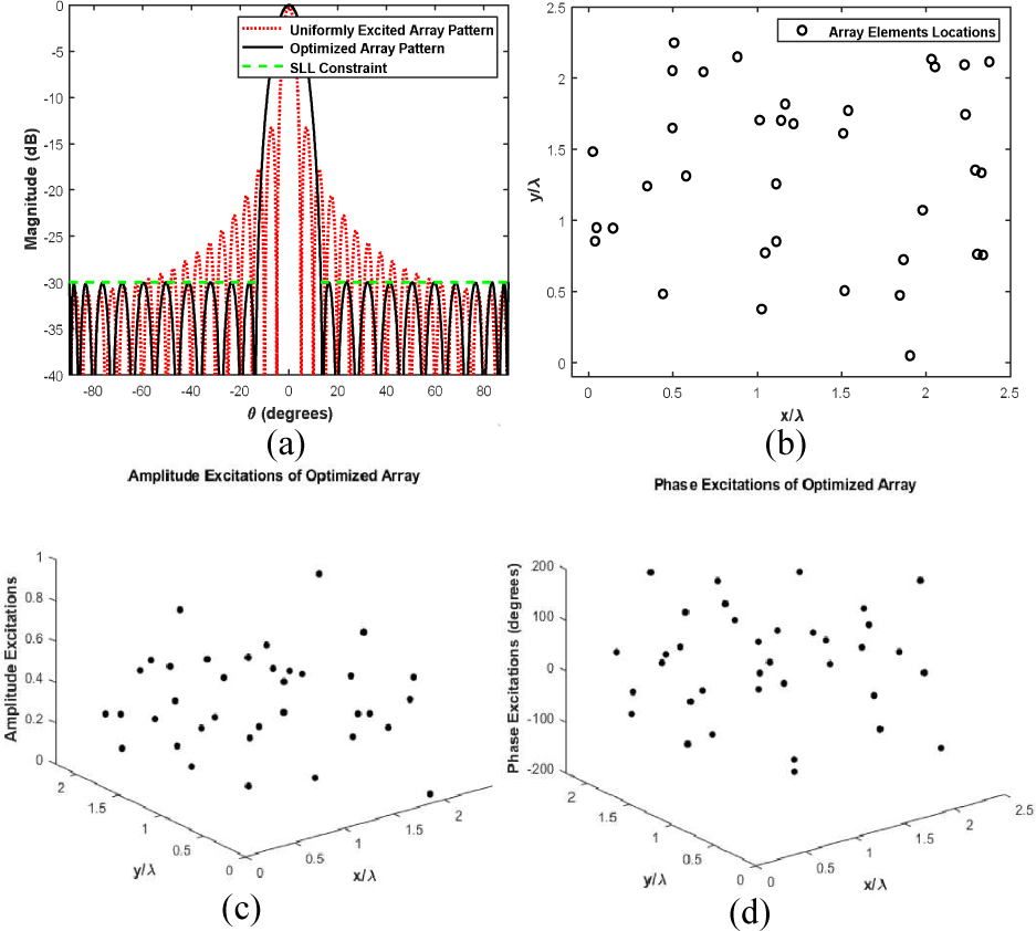
Figure 9: (a) Optimized pattern of the random array with 66 elements for SLL = 30 dB, (b) its element locations, (c) excitation amplitudes, and (d) phases.
Finally, Fig. 10 shows the variations of the minimum feasible beam width and the directivities for different values of the given SLL. It can be seen that the higher SLL results in a narrower beam width. These results fully confirm the effectiveness of the convex optimization algorithm for designing linear, planar, and random arrays.
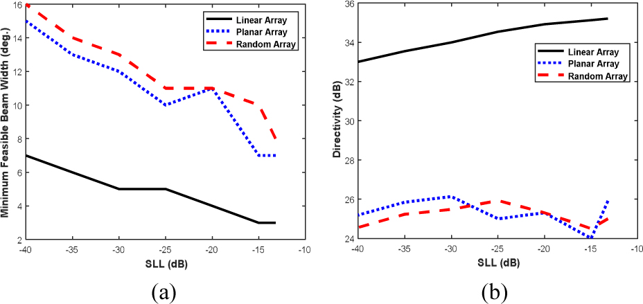
Figure 10: (a) Variation of minimum SLL and (b) directivity.
4 CONCLUSION
Convex optimization has been used effectively to obtain the desired radiation patterns of the linear, planar, and random arrays by optimizing the excitation amplitudes and phases of the array elements subject to either finding the minimum possible sidelobe level for a given beam width pattern or finding the minimum possible beam width for a given sidelobe level. From the results of the linear, planar, and random array configurations, it has been shown that a much lower SLL can be obtained for higher beam width values at the cost of lower directivities. Moreover, the performance of the linear arrays was found to outperform in terms of minimum feasible SLL for a given narrow beam width compared to the other two configurations. This is mainly due to the linear array has wider space diversity. On the other hand, the three array configurations perform well and provide feasible minimum beam width for relatively high SLL. These results fully confirm the capability of the suggested two optimization constraint methods.
REFERENCES
[1] J. R. Mohammed, “Performance optimization of the arbitrary arrays with randomly distributed elements for wireless sensor networks,” International Journal of Telecommunication, Electronics, and Computer Engineering, vol. 11, no. 4, pp. 63-68, 2019.
[2] C. A. Balanis, Antenna Theory: Analysis and Design, 4th ed., Wiley, 2016.
[3] J. R. Mohammed and K. H. Sayidmarie, “Sensitivity of the adaptive nulling to random errors in amplitude and phase excitations in array elements,” International Journal of Telecommunication, Electronics, and Computer Engineering, vol. 10, no. 1, pp. 51-56, 2018.
[4] P. Daniele, “On the trade-off between the main parameters of planar antenna arrays,” Electronics, vol. 9, 2020.
[5] J. R. Mohammed and K. H. Sayidmarie, “Synthesizing asymmetric sidelobe pattern with steered nulling in non-uniformly excited linear arrays by controlling edge elements,” International Journal of Antennas and Propagation, vol. 2017, 2017.
[6] J. R. Mohammed, “Obtaining wide steered nulls in linear array patterns by controlling the locations of two edge elements,” AEÜ International Journal of Electronics and Communications, vol. 101, pp. 145-151, 2019.
[7] J. R. Mohammed, “Optimal null steering method in uniformly excited equally spaced linear array by optimizing two edge elements,” Electronics Letters, vol. 53, no. 13, pp.835-837, 2017.
[8] J. R. Mohammed, “Element selection for optimized multi-wide nulls in almost uniformly excited arrays,” IEEE Antennas and Wireless Propagation Letters, vol. 17, no. 4, pp. 629-632, 2018.
[9] J. R. Mohammed and K. H. Sayidmarie, “Sidelobe cancellation for uniformly excited planar array antennas by controlling the side elements,” IEEE Antennas and Wireless Propagation Letters, vol. 13, pp. 987-990, 2014.
[10] L. Wen-Pin and C. Fu-Lai, “Null steering in planar array by controlling only current amplitudes using genetic algorithms,” Microwave and Optical Technology Letters, vol. 16, no. 2, pp. 97-103,1997.
[11] J. Robinson and Y. Rahmat-Samii, “Particle swarm optimization in electromagnetics,” IEEE Trans. Antennas Propag., vol. 52, no. 2, pp. 397-407, 2004.
[12] M. Raíndo-Vázquez, A. Salas-Sánchez, J. Rodríguez-González, M. López-Martín, and F. Ares-Pena, “Optimizing radiation patterns of thinned arrays with deep nulls fixed through their representation in the schelkunoff unit circle and a simulated annealing algorithm, Sensors, vol. 22, 2022. https://doi.org/10.3390/s22030893
[13] E. Aksoy and E. Afacan, “Planar antenna pattern nulling using differential evolution algorithm,” AEU Int. J. Electron. Commun., vol. 63, pp. 116-122, 2009.
[14] A. Akdagli, K. Guney, and D. Karaboga, “Touring ant colony optimization algorithm for shaped-beam pattern synthesis of linear antenna,” Electromagnetics, vol. 26, no. 8, pp. 615-628, 2006.
[15] Y. Qu, G.S. Liao, S. Q. Zhu, and X.Y. Liu, “Pattern synthesis of planar antenna array via convex optimization for airborne forward looking radar,” Progress in Electromagnetics Research, vol. 84, pp. 1-10, 2008.
[16] O. M. Bucci, M. D’Urso, and T. Isernia, “Exploiting convexity in array antenna synthesis problems,” IEEE Radar Conference, Rome, Italy, pp. 1-6, 2008, doi: 10.1109/RADAR.2008.4720832.
[17] E. Kurt, S. Basbug, and K. Guney. “Linear antenna array synthesis by modified seagull optimization algorithm,” Applied Computational Electromagnetics Society (ACES) Journal, vol. 36, no. 12, pp. 1552-1562, 2022.
[18] A. Z. Elsherbeni and M. J. Inman, “Antenna design and radiation pattern”, Applied Computational Electromagnetics Society (ACES) Journal, vol. 18, no. 3, pp. 26-32, Jun. 2022.
BIOGRAPHIES

Jafar R. Mohammed received B.Sc. and M.Sc. Degrees in Electronics and Communication Engineering in 1998 and 2001, respectively, and a Ph.D. degree in Digital Communication Engineering in Nov. 2009. He was a visiting lecturer in the faculty of Electronics and Computer Engineering at the Malaysia Technical University Melaka (UTeM), Melaka, Malaysia in 2011 and the Autonoma University of Madrid, Spain in 2013. He is currently a Professor and Vice Chancellor for Scientific Affairs at Ninevah University, Mosul, Iraq. He authored more than 70 papers in international refereed journals and conference proceedings. Also, he edited the book titled ”Array Pattern Optimization” published by IntechOpen in 2019. His main research interests are in the area of Digital Signal Processing and its applications, Antenna, and Adaptive Arrays. In 2011, He is listed in Marquis, Who’s Who in Science and Engineering (Edition 28). In 2018, he has been selected for the Marquis Who’s Who Lifetime Achievement Award.

Rana R. Shaker received a B.Sc. degree in Communication Engineering from College of Electronic Engineering, Ninevah University. She is currently pursuing her Master’s degree at the same university. Her research interests include antenna arrays and array pattern optimization.
ACES JOURNAL, Vol. 37, No. 7, 811–816.
doi: 10.13052/2022.ACES.J.370708
© 2022 River Publishers