Modeling the Performance Impact of Cubic Macro Cells Used in Additively Manufactured Luneburg Lenses
Brian F. LaRocca and Mark S. Mirotznik
1Department of the Army, Aberdeen Proving Ground, Aberdeen, MD 21005, USA
brian.f.larocca.civ@army.mil
2Electrical Engineering Department, University of Delaware, Newark, DE 19716, USA
mirotzni@udel.edu
Submitted On: May 25, 2022; Accepted On: September 29, 2022
ABSTRACT
Finite Element Analysis (FEA) is used to determine the sensitivity of feed placement on a Luneburg lens (LL) having large scale cubic discretization of its permittivity distribution. This is of practical importance for lenses fabricated using additive manufacturing, allowing accurate prediction of performance, and potentially reducing overall print time. It is shown that the far-field relative side lobe level (RSLL) is most sensitive to this form of discretization, and the impact to multi-feed and single-feed applications is considered. It is shown that for single-feed applications, large cubic macro cells are beneficial and provide a RSLL above that achieved with the continuous and non-uniform shelled counterparts.
Index Terms: 3D printing, finite element analysis, Luneburg lens, unit cells.
I. INTRODUCTION
While spatially graded dielectrics, also known as graded-index (GRIN) structures, are popular devices in optics and photonics, they have historically been used less frequently at radio frequencies (RF). However, there has been a recent surge of interest in using RF GRIN antennas as low-cost alternatives to phased arrays. One of the most popular RF GRIN structures is the well-known LL [1-4]. The LL is a spherical device in which every point on the surface is the focal point of a plane wave incident from the opposing surface. This unique property is leveraged to realize passive beam steering antennas capable of directing a single or multiple beams over wide scan angles.
While the LL concept has been known for nearly 80 years [1], our ability to reliably manufacture them has been aided by recent advancements in additive manufacturing (AM) technologies and materials. Prior to AM, fabricating a structure with spatially graded dielectric properties was an expensive and challenging manufacturing problem.
Over the last eight years, a host of papers have been published on the use of AM to fabricate the LL and other GRIN devices [5-11]. While these previous studies have demonstrated AM’s ability to fabricate functional RF GRIN lenses, what has not been well characterized is the impact of non-spherical discretization larger than a small fraction of a wavelength.
In this paper, a full wave computational study is presented that quantifies the effect of introducing a discretization beyond that of the unit cell scale, in other words, at the macro cell scale. As illustrated in Fig. 1, it considers a
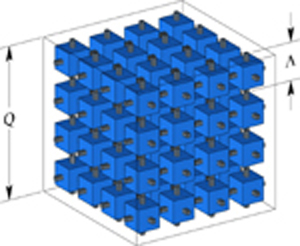
Figure 1: A macro cell being composed of an integral number of identical unit cells such as depicted in Fig. 2.
cubic macro cell that is comprised of an integral number of identical unit cells such as that shown in Fig. 2. On the surface of the lens, the cells are

Figure 2: A typical Unit cell. The effective permittivity of the cell is controlled by manipulating the volume of printed material , to the total volume of the cell .
allowed to conform to the spherical surface, but otherwise the lens is comprised of identically sized macro cells, each with a permittivity equal to that of the underlying unit cells. Visualizations resulting from this discretization are shown in Fig. 3.
The ability to additively manufacture the sub-wavelength unit cell lattice depicted in Fig. 1 has been successfully demonstrated by the researchers in [7] using the polymer jetting approach. In that research, the authors designed and built a 60 mm radius LL for operation at 10 GHz.
The material used in [7] is a UV-curable acrylic polymer of with a loss tangent of 0.02. For any given polymer, the authors in [11] determine the maximum useful radius of an additively manufactured LL by applying the constraint that the main beam of the radiation pattern contain at least of accepted power. According to their results, a LL constructed with the polymer used in [7] may only have a maximum useful radius of . To take advantage of the RSLL improvement that the macro cell quantization affords as shown in Table 1, the AM technique known as Fused Deposition Modeling (FDM) is required, due to the much lower loss of engineering thermoplastics. According to [11], FDM using Polycarbonate can produce a LL with a maximum useful radius of . The structure in Fig. 1 does require a dual nozzle FDM printer to dispense a support thermoplastic along with the Polycarbonate. Once the heated thermoplastic cools and hardens, the support plastic is flushed from the structure with water.
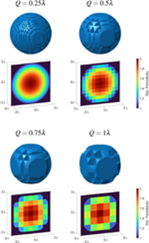
Figure 3: Visualizations of macro cell LL as the cell edge length , is varied from to . Radius of lens is held constant at . Below each 3D model is a 2D slice through the center of the lens and colorized to reveal the relative permittivity distribution.
II. MODELING AND ANALYSIS
A. Simulation and model parameters
The 3D FEA of this research is performed using the COMSOL Multiphysics software [17] equipped with the RF Module. A sketch identifying the components of the physical model, is provided in Fig. 4. Depending upon the stage of analysis, the lens may have a permittivity distribution that is either continuous or discretized into spherical layers or macro-cell cubes.
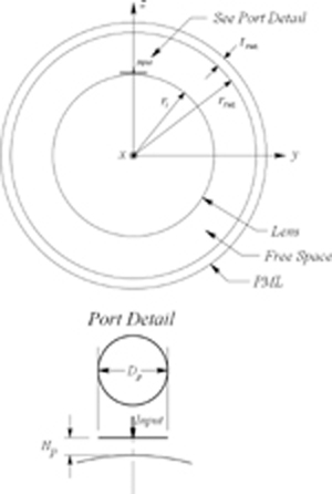
Figure 4: Sketch of model used for this research consisting of a spherical LL, a circular waveguide feed, and a spherical Perfectly Matched Layer (PML).
The waveguide feed is modeled as a circular port that matches the EIA WC59 designation with an internal diameter of 0.594 inch. The port height is fixed at 0.25 mm. The lowest order mode for a circular waveguide is followed by [18]. To ensure operation in the mode, the operating frequency is set as follows:
| (1) |
where GHz and GHz. The simulation uses GHz yielding a free-space wavelength of mm.
A behavioral model is used to implement Left Hand Circular (LHC) polarization for the waveguide feed. This is accomplished by defining two linearly polarized ports on a single circular boundary, each with a polarization axis that is orthogonal to the other. An appropriate phase difference is then applied to ensure counterclockwise field rotation when viewed along the direction of wave travel. The resulting polarization vector is written as:
| (2) |
and , where is the unit propagation vector.
A spherical coordinate system as depicted in Fig. 5 is used throughout. Note that when describing far-field patterns, the radial distance is irrelevant, and not provided.
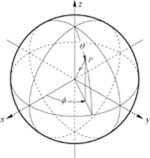
Figure 5: Spherical coordinate system used throughout.
B. Quantization of lens permittivity
The LL studied in this paper has a quantized permittivity distribution using what is referred to herein as macro cells. Other than conforming to the spherical lens surface, macro cells are modeled as equal sized dielectric cubes that are homogeneous, isotropic, and lossless. The permittivity throughout a given macro cell is, therefore, constant and is specified knowing the center point of the representative cube.
As a matter of convenience, the quantized permittivity distribution throughout the lens is generated indirectly by first mapping the set of Finite Element mesh vertices within the lens to the much smaller set of macro cell center points. Allowing to represent the , , and coordinates of a given mesh vertex, to represent the corresponding coordinates associated with the center point of the enclosing macro cell, and to represent the macro cell edge length, then:
| (3) |
where is to be understood as the standard “round to nearest integer” function. Once (3) is used to perform the mapping from mesh vertices to macro cell center points, i.e., , the relative permittivity is computed using the standard Luneburg equation. We first define the distance between the lens center to any macro cell center point as being . Then, for a lens of radius that is centered at the origin of the mesh coordinate system:
| (4) |
The sequential application of (3) then (4) achieve the desired mapping . The if statement in (4) is necessary since there are always macro cells that protrude through the lens surface and have their center point outside of the lens surface. For these cases, the otherwise clause avoids inadvertently modeling an less than 1.0.
In Fig. 6, the relative permittivity distribution of a continuous LL is presented along

Figure 6: LL relative permittivity distributions: (a) the continuous version, and in (b) the discrete counterpart.
with that of the discretized version. For the lens shown, and, where is a specified free space wavelength. The effective radius of discrete version along the coordinate axes is shorter than may be expected, and in fact, is equal to . This is a result of groupings of macro cells having an equal to that of free space. These can be thought of as virtual cells; thus, time nor material need be expended to produce them. For the lens shown, there are 30 out of 925 total cells that are virtual, i.e., have an . With reference to the separation between the lens and the feed port in the detail of Fig. 4, is always measured relative to the virtual surface of the LL residing at .
To relate the concept of the macro cell to a fabricable device, we discussed the use of a much smaller sub-wavelength lattice structure as illustrated in Fig. 1 and Fig. 2. There the dimensions of the lattice are depicted by , where is much smaller than the wavelength, i.e., . A 3D array of these smaller structures represents a single macro cell (see Fig. 1) with an effective homogenous permittivity. This is a common approach when fabricating a LL using additive manufacturing methods.
The relationship between the effective permittivity of the macro cell and the smaller array of sub-wavelength geometries have been described in several of the references including [7] and are determined using effective media theory. Our full wave FEA model and analysis is at the macro cell scale. By doing so reduces the peak memory requirement by a factor of and enables meaningful 3D FEA on practical engineering workstations. In fact, the largest LL studied requires a peak memory requirement of 90 GB using the COMSOL RF module.
C. Far-field parameters
The ideal feed for a continuous LL is a point source placed on the surface of the lens. Furthermore, the radiation pattern of the point source is required to have a cosine shape with its peak oriented towards the center of the lens [16]. When this is the case, the system is said to have an aperture efficiency equal to 1. In this context, is interpreted as:
| (5) |
where represents the effective or achieved aperture, and is the physical area of the lens aperture, being [3]. In other words, for the ideal system:
| (6) |
The system gain is defined as the ratio of to the aperture of an isotropic reference , where:
| (7) |
Thus [3]:
| (8) |
Combining (6) and (8), the boresight gain for a continuous LL with an ideal point source feed is therefore:
| (9) |
In the analysis conducted herein, however, the lens feed is modeled as a circular waveguide. Under this feed condition, the aperture efficiency is less than unity and is dependent upon the effective aperture of the waveguide [16]. We therefore use (5) to write:
| (10) |
and upon combining (8) and (10), we have:
| (11) |
A range of spherical Luneburg lenses with a continuous permittivity distribution having radii from to in increments are evaluated. With each near-field solution, the COMSOL RF module generates the corresponding 3D far-field radiation pattern. Afterwards, the pattern is analyzed in MATLAB where gain is extracted, and the Relative Side Lobe Level (RSLL) and Half Power Beam Width (HPBW) are computed. In this research, the RSLL is taken as the difference in decibels between the gain of the main lobe and the highest side lobe [2].
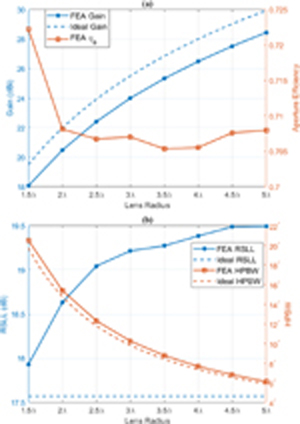
Figure 7: Continuous LL performance vs lens radius. Solid traces are FEA results and dashed traces are derivedfrom (12).
The gain and aperture efficiency, , are plotted versus lens radius in Fig. 7 (a), and the RSLL and HPBW are plotted in Fig. 7 (b). Additionally, the respective gain, RSLL, and HPBW for the ideal point source fed continuous lens is provided in each case. For this purpose, (12) provides the analytical expression of the far-field gain [16], and MATLAB post-processing computes the corresponding RSLL and HPBW. For these calculations, the lens radius is sampled every to ensure the resulting curves are smooth. Moreover, when compared to the ideal point source fed lens, the FEA results show lower gain, a slightly wider beam width and a better RSLL. Note that in (12), represents the Bessel function of the first kind of order one, and is the free-space phase constant being equal to . With the feed point source located at , the boresight gain evaluated with (12) is , and this value is identical to that provided earlier in (9).
| (12) |
Examination of Fig. 7 (b) reveals that the RSLL derived from (12) appears to be constant and is therefore independent of the lens radius . Although this result may not be deduced easily from (12), it is explicitly demonstrated for two values of in Fig. 8. The ratio between the lens radius used in Fig. 8 (b) and Fig. 8 (a) is . From (9), we therefore expect a 20 dB difference in boresight gains between the two, and this is indeed observed in Fig. 8. However, the RSLL is seen to remain constant at approximately 17.6 dB. Using inductive reasoning, we conclude that the RSLL of (12) is independent of .
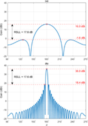
Figure 8: RSLL measurement of radiation pattern specified by (12). In (a) and in (b) .
D. Non-uniform shell
The prevalent method of fabricating the LL is to use a layered approach as depicted in Fig. 9. Using this construction method, a spherical dielectric core is surrounded by a series of spherical dielectric shells. The core and surrounding shells are homogeneous, with their respective permittivity and radius chosen to mimic a continuously graded LL. The optimum selection of these parameters proceeds once the number of layers is chosen and includes both closed form expressions [12] and iterative methods [13-15]. The equations of [12] are repeated here as a point of reference. They are simple and yet optimally approximate the continuous LL distribution for a given number of layers.

Figure 9: Example of a multiple layer spherical LL with wedge cut out to expose interior construction. The central core has radius , and the five surrounding shells have outer radii of through .
We begin with the continuous LL permittivity distribution. Using to represent the radial distance from the lens center to any point within the lens, and to represent the LL radius, the relative permittivity at that point is given by:
| (13) |
We now number the individual layers from 1 to , where corresponds to the core, and corresponds to the outer most layer. From [12], the relative permittivity of layer is given by:
| (14) |
and the outer radius of layer is given by:
| (15) | ||
The effectiveness of (14) and (15) in approximating (13) is demonstrated in Fig. 10 (a) for and in Fig. 10 (b) for . From these two plots, it is observed that as the magnitude of slope of (13) increases, the layers become thinner and the permittivity contrast between layers decreases.
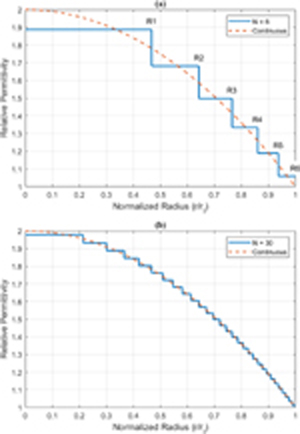
Figure 10: Optimum layer relative permittivity versus normalized radius for in (a) and for in (b). The layer radii to in (a) correspond to similarly marked layers in Fig. 9.
From Fig. 10, it is obvious that as the number of layers increases, the discrete permittivity profile becomes a better approximation to the continuous LL. However, large is accompanied by stringent requirements in terms of precision for both layer permittivity and curvature. It is therefore necessary to select the minimum at which design goals are still met. As demonstrated by the FEA results shown in Fig. 11, the radiation pattern of a lossless six-layer LL accurately approximates that of the continuous counterpart. In fact, the difference in gain, RSLL, and HPBW between the two are:
| (16) | ||
where , , and refer to the metrics of the six-layer lens, and , , and to that of the continuous version. It is not surprising that the performance of lens is slightly less than the continuous prototype, and given reasonable manufacturing tolerances, increasing the layer count may not be beneficial.
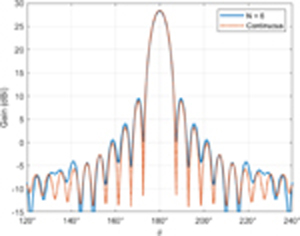
Figure 11: FEA results providing gain comparison between a 6 layer LL and a continuous LL. Both lenses are modeled with lossless dielectrics and have a lens radius of .
Fig. 12 provides insight into why is a good choice for a layered LL that is designed using (14) and (15). By substituting for in (13) and integrating with respect to , we derive the area under the continuous LLcurve:
| (17) | ||
Conversely, the area under the discrete approximation for a given number of layers , is obtained using:
| (18) |
A useful relative error metric between the continuous version of (13) and the discrete level approximation, can then be defined [12] as:
| (19) |
In Fig. 12, both and are plotted for layers. The constant is plotted as a dashed red horizontal asymptote, and is a solid orange trace that approaches for large . Referring to the vertical marker at layers, it is seen that the error increases rapidly to the left and slowly to the right. Depending upon tooling capabilities and material availability, the engineer would probably select a design having or 7 layers.
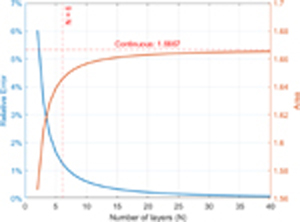
Figure 12: Area under discrete LL permittivity distribution and the relative error versus the number of layers .
The results presented in Fig. 12 for discrete spherical shells agree with previously reported results given in [12-15]. This analysis provides a good baseline to compare results from the cubical macro-cell discretization described in the subsequent sections.
E. Port location sweep
In multibeam applications, antenna feeds are distributed across the lens surface, and it is therefore necessary to ascertain how feed location impacts the far-field radiation pattern. For the case of the spherical shell discretization, presented in the previous section, the radiation patterns are independent of feed location due to symmetry. However, this is not true for the case of the cubical macro-cells shown in Fig. 3.
Assuming feeds are facing the lens and radially directed, feed location is given by the spherical coordinate , where the subscript is used to avoid confusion with far-field coordinates. The port height is fixed at 0.25 mm. The permittivity distribution of a LL with a non-zero macro cell edge length , does not contain a strict spherical symmetry. Thus, performance should be expected to depend upon and . To establish this dependence, FEA is performed on lenses over a range of and , while the of a single waveguide feed is swept. Given the symmetry of the lens, the sweep need only cover and . An angular resolution of is selected, and therefore separate FEA runs are required to complete a single combination. With each run, far-field data is saved to a unique file. The files are post-processed in MATLAB, where boresight gain and Axial Ratio (AR) are extracted, and the RSLL, HPBW, and Polarization Loss Factor (PLF) are computed.
An example RSLL computation over a sweep for the lens is shown in Fig. 13. Because of the relatively large value of , there is an appreciable spread of values. It is also interesting to note that for , and several other feed locations, the lens outperforms the continuous counterpart, i.e., the lens . Using the value read from the plot in Fig. 7 (b), this difference is as great as dB.
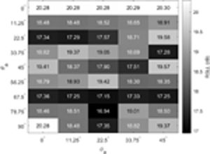
Figure 13: RSLL matrix for the sweep of lens . The spread in RSLL is 3.36 dB, however, there are multiple values that are better than that of the continuous reference.
Lens radius varies from to in steps, and cell size varies from to in steps. In Fig. 14, the lens is shown along with an overlay of the port grid and the circular port boundary; both drawn to scale. The feed location in this example yields the worst case RSLL for this lens. The radiation pattern for the given port location is also shown.
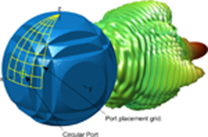
Figure 14: Port placement is swept over a sector grid suspended above the lens surface.
Considerable axial asymmetry exists in the far-field radiation patterns for lenses with large . The RSLL calculation requires that the peak side lobe be identified, and the method employed slices the 3D pattern into a sequence of 2D cuts. In turn, each cut is analyzed in MATLAB using the standard findpeaks() function, with additional code to handle the circular nature of . The cut with the largest peak side lobe is recorded and used for determination of the RSLL of the pattern overall. A similar procedure is also used to determine the HPBW. An example pattern is shown in Fig. 15.
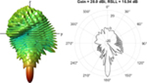
Figure 15: The RSLL is determined by examining individual 2D cuts through the full 3D radiation pattern. Cuts are taken every and are sampled with a resolution of . This pattern is for the lens with feed location of .
III. RESULTS
Results are presented as a series of contour plots that describe how the edge length of a macro cell impacts the far-field parameters, as the lens radius is varied. Best-and worst-case results are provided, representing data taken only at the feed location that produces the respective extremum. Results are shown for the far-field parameters of gain in Fig. 16, RSLL in Fig. 17, AR in Fig. 18, and HPBW in Fig. 19.
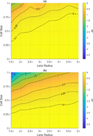
Figure 16: Loss in gain due to quantization: (a) best case, and in (b) worst case.
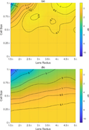
Figure 17: Loss in RSLL due to quantization: (a) best case, and in (b) worst case. Best case includes areas where loss is negative. This means that the best case RSLL in these areas is better than the continuous counterpart lens.

Figure 18: Worst case increase in AR due to quantization. Best case increase in AR is for all modeled and is not plotted.
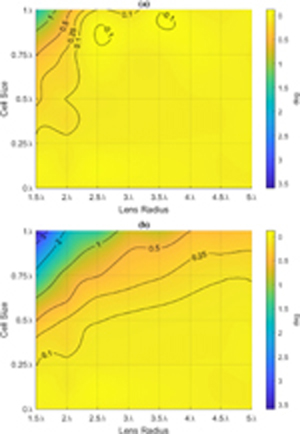
Figure 19: Increase in HPBW due to quantization: (a) best case, and in (b) worst case. Best case includes an area where increase is slightly negative. This means that the best case HPBW in this area is narrower than the continuous counterpart lens.
For gain and RSLL, the impact of is represented as a loss. The worst-case loss is equal to the gain or RSLL of the counterpart continuous lens, minus the minimum value of the respective matrix for a given . The best-case loss is equal to the gain or RSLL of the counterpart continuous lens, minus the maximum value of the respective matrix for a given . The gain vs. for the continuous counterpart is shown in Fig. 7 (a) and it’s RSLL in Fig. 7 (b).
For HPBW, the impact of is represented as an increase in beam width. The worst-case increase is equal to the maximum value of the HPBW matrix for a given , minus the HPBW of the counterpart continuous lens. The HPBW vs. for the continuous counterpart is plotted in Fig. 7 (b). In the case if AR, the impact is just a larger value of AR. It is equal to the maximum value of the AR matrix for a given less unity, since the AR of the continuous counterpart is exactly 1 for LHC polarization. The best-case increase in beam width is equal to the minimum value of the HPBW matrix for a given , minus the HPBW of the counterpart continuous lens. The best-case impact to AR is equal to the minimum value of the AR matrix for a given less unity. However, for the range of and modeled, the best-case impact to AR , and is therefore not plotted in Fig. 18.
The contour plots in Figs. 16–19 appear to represent the data as continuous values. However, the underlying data is an array, where is the number of values that have been modeled, and is the number of values modeled. For the results presented here, and . To produce the intervening data, the MATLAB curve fitting toolbox is used to smoothly fit a surface to the available data points. Out of numerous possibilities, the thin-plate spline surface fitter is chosen for this purpose, since it produces a smooth surface and has favorable extrapolation properties [19]. The results shown here do not include extrapolated data.

Figure 20: Histogram of best feed placements.
Moreover, the contour plots are relative to the FEA results for a LL with . Being relative to the continuous counterpart, these results directly show the impact due to quantization.
IV. DISCUSSION
The results presented in Section III are in terms of best-and worst-case impacts. Both cases are necessary, since the radiation pattern is dependent upon feed position for a LL with . For multi-feed designs, the results provide the maximum spread in performance metrics over the set of feeds. If a feed pattern is sparse, it may be possible to optimize performance by avoiding certain feed locations. For single-feed designs, the worst-case impacts are ignored, and the feed should be located at an optimum position. In many instances, optimizing the dynamic range is paramount, which implies that the feed placement should optimize the RSLL. As you can see in Fig. 17 (a), this can result in a dynamic range improvement of over 1 dB for a radius lens with , relative to the continuous LL.
Table 1: Summary of discretization impact for a LL with a radius of . All values are relative to FEA results for a continuous LL. Negative loss or growth indicates that the impact is beneficial. For each edge length , the impacts are shown in two rows: top row is best case, bottom row is worst case
| Lens | Gain | RSLL | HPBW | AR |
|---|---|---|---|---|
| Loss (dB) | Loss (dB) | Growth | Growth | |
| 6 Layer Shell | 0.13 | 0.66 | 0 | |
| 0 | 0.01 | 0 | ||
| 0.01 | 0.05 | 0 | ||
| 0.04 | -0.12 | 0 | ||
| 0.11 | 0.34 | 0.02 | ||
| 0.05 | -0.10 | 0 | ||
| 0.38 | 1.83 | 0.03 | ||
| 0.40 | -0.81 | 0 | ||
| 0.91 | 2.55 | 0.06 |
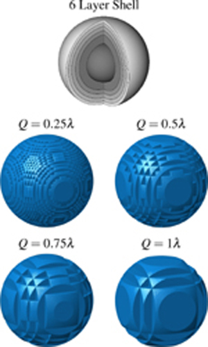
Figure 21: Discrete versions of LL: non-uniform layered shell and cubic macro cell. Radius of lenses shown is . Performance of this set of five lenses is summarized in Table 1.
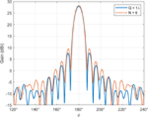
Figure 22: Comparison of radiation patterns between best case and 6-layer shell LLs. Both lenses have a radius of . The difference in the RSLL between the two is 1.47 dB.
The best-case feed position , varies with cell size and lens radius . A histogram that simply counts the number of times a particular grid position is the best location modeled is provided in Fig. 20. This histogram only considers the 32 lenses that have a non-zero cell size. Placement at includes 18 occurrences, and thus accounts for approximately the lenses modeled.
Table 1 summarizes the quantization impact for a LL having a radius of . For further context, it includes the 6-layer optimal shell design of Section II.D. Also, the five lenses included in this summary are shown in Fig. 21. From Table 1, it is seen that the shell design has similar performance to that of the worst-case lens. Thus, for multi-feed applications, the macro cell lens would at worse perform the same as the 6-layer design. For single feed applications, however, the lens provides 1.47 dB increased dynamic range over the 6-layer design. This is demonstrated in Fig. 22, where the radiation pattern of each is juxtaposed.
V. CONCLUSION
The far-field parameters of gain, RSLL, HPBW, and AR are not equally sensitive to the cubic macro cell quantization of the LL permittivity distribution. Observing the worst-case results in Figs. 16–19, a reasonable conclusion is that the ordering from least to greatest sensitivity is: AR, HPBW, gain, then RSLL.
RSLL sensitivity to feed location increases as the macro cell edge length Q is increased. Over the range of investigated, this may limit for multi-feed applications. In this regard, it is shown that a lens with and has a worst case RSLL that is 0.32 dB better than a similarly sized 6-layer non-uniform shell design. For single-feed use, and depending upon the lens radius, larger macro cells are beneficial and increase RSLL further. It is found that a lens with and has an RSLL that is 0.81 dB better than a continuous LL and 1.47 dB better than the 6-layer non-uniform shell design.
Moreover, the results presented in Figs. 16–19 condense the effect of feed location on far-field parameter sensitivity into best-and worst-case contour plots. Over the range of and investigated, the plots allow for determination as to the severity of performance impact and, therefore, inform decisions regarding the maximum macro cell size that can be tolerated for agiven .
REFERENCES
[1] R. K. Luneburg, Mathematical Theory of Optics, Brown University Press, Providence, 1944.
[2] B. Edde, RADAR – Principles, Technology, Applications, Prentice Hall PTR, New Jersey, 1993.
[3] R.C. Johnson, Antenna Engineering Handbook, McGraw-Hill, New York, 1993.
[4] Y. T. Lo and S. W. Lee, Antenna Handbook-Vol. II Antenna Theory, Van Nostrand Reinhold, New York, 1993.
[5] C. Babayigit, A. S. Evren, E. Bor, H. Kurt, and M. Turduev, “Analytical, numerical, and experimental investigation of a Luneburg lens system for directional cloaking,” Phys. Rev., A 99, 043831, Apr. 2019.
[6] Z. Larimore, S. Jensen, A. Good, J. Suarez and M. S. Mirotznik, “Additive manufacturing of Luneburg lens antennas using space filling curves and fused filament fabrication,” IEEE Transactions on Antennas and Propagation, vol. 66, no. 6, pp. 2818-2827, Jun. 2018.
[7] M. Liang, W. R. Ng, K. Chang, K. Gbele, M. E. Gehm, and H. Xin, “A 3-D Luneburg lens antenna fabricated by polymer jetting rapid prototyping,” IEEE Transactions on Antennas and Propagation, vol. 62, no. 4, pp. 1799-1807, Apr. 2014.
[8] C. Wang, J. Wu, and Y. Guo, “A 3-D-printed wideband circularly polarized parallel-plate luneburg lens antenna,” IEEE Transactions on Antennas and Propagation, vol. 68, no. 6, Jun. 2020.
[9] S. Lei, K. Han, X. Li, and G. Wei, “A design of broadband 3-D-printed circularly polarized spherical Luneburg lens antenna for X-band,” IEEE Antennas and Wireless Propagation Letters, vol. 20, no. 4, Apr. 2021.
[10] B. LaRocca, M. S. Mirotznik, “Modeling the performance impact of anisotropic unit cells used in additively manufactured Luneburg lenses,” Applied Computational Electromagnetics Society (ACES) Journal, vol. 37, no. 1, pp. 50-57, 2022.
[11] B. LaRocca, M. S. Mirotznik, “An empirical loss model for an additively manufactured Luneburg lens antenna,” Applied Computational Electromagnetics Society (ACES) Journal, vol. 37, no. 5, pp. 554-567, 2022.
[12] C. S. Silitonga, Y. Sugano, H. Sakura, M. Ohki, and S. Kozaki, “Optimum variation of the Luneberg lens for electromagnetic scattering calculations,” International Journal of Electronics, vol. 84, no. 6, pp. 625-633, 1998.
[13] H. Mosallaei and Y. Rahmat-Samii, “Nonuniform Luneburg and two-shell lens antennas: Radiation characteristics and design optimization,” IEEE Transactions on Antennas and Propagation, vol. 49, no. 1, pp. 60-69, Jan. 2001.
[14] B. Fuchs, L. Le Coq, O. Lafond, S. Rondineau, and M. Himdi, “Design optimization of multishell Luneburg lenses,” IEEE Transactions on Antennas and Propagation, vol. 55, no. 2, pp. 283-289, Feb. 2007.
[15] H. Chou, Y. Chang, H. Huang, Z. Yan, T. Lertwiriyaprapa, and D. Torrungrueng “Optimization of three-dimensional multi-shell dielectric lens antennas to radiate multiple shaped beams for cellular radio coverage,” IEEE Access, vol. 17, 2019.
[16] G. Guo, Y. Xia, C. Wang, M. Nasir, and Q. Zhu, “Optimal radiation pattern of feed of Luneburg lens for high-gain application,” IEEE Transactions on Antennas and Propagation, vol. 68, no. 12, pp. 8139-8143, Dec. 2020.
[17] COMSOL Multiphysics® v. 5.6. www.comsol.com. COMSOL AB, Stockholm, Sweden.
[18] O. P. Gandhi, Microwave Engineering and Applications, Pergamon Press, New York, 1985.
[19] MATLAB, ver. 2021a, The Mathworks Inc., Natick, Massachusetts, 2021.
BIOGRAPHIES

Brian F. La Rocca received B.S.E.E and M.S.E.E degrees from New Jersey Institute of Technology, Newark, NJ, USA in 1985 and 2000, respectively. From 1985 to 1996, he worked in industry, from 1996 to 2004 as a government contractor, and from 2004 to present as a civilian engineer with the Dept. of the Army at Ft. Monmouth, NJ, USA and Aberdeen Proving Ground, MD, USA. He received his Ph.D. degree in electrical engineering from the University of Delaware, Newark, DE, USA in the summer of 2022.

Mark S. Mirotznik (S’87–M’92–SM’11) received his B.S.E.E. degree from Bradley University, Peoria, IL, USA, in 1988, and his M.S.E.E. and Ph.D. degrees from the University of Pennsylvania, Philadelphia, PA, USA, in 1991 and 1992, respectively. From 1992 to 2009, he was a Faculty Member with the Department of Electrical Engineering, The Catholic University of America, Washington, DC, USA. Since 2009, he has been a Professor and an Associate Chair for Undergraduate Programs with the Department of Electrical and Computer Engineering, University of Delaware, Newark, DE, USA. He holds the position of Senior Research Engineer with the Naval Surface Warfare Center, Carderock Division. His current research interests include applied electromagnetics and photonics, computational electromagnetics, multifunctional engineered materials, and additive manufacturing.
ACES JOURNAL, Vol. 37, No. 10, 1077–1088
doi: 10.13052/2022.ACES.J.371008
© 2022 River Publishers