Removing the Froissart Doublets in a Rational Interpolation Based on Loewner Matrix

Haobo Yuan${}^{\mathbf{\text{1}}}$, Jungang Ren${}^{\mathbf{\text{1}}}$, Yujie Li${}^{\mathbf{\text{2}}}$, and Xiaoming Huang${}^{\mathbf{\text{1}}}$

¹National Key Laboratory of Antenna and Microwave Technology
Xidian University, Xi’an, 710071, China
hbyuan@mail.xidian.edu.cn, renjungang20@gmail.com, hxm_0314@126.com

²Hangzhou Institute of Technology
Xidian University, Hangzhou, 311200, China
liyujie3128@163.com

Submitted On: June 22, 2022; Accepted On: July 13, 2022

ABSTRACT

In order to implement wide band frequency sweeping, the S-parameters can be fitted with an adaptive rational interpolation based on Loewner matrix. However, the errors in the sampling data may lead to Froissart doublets, which look like spikes in the curve. In this paper, a novel technique is proposed to remove these doublets. At first, the rational expression is converted into the sum of partial fractions by solving two generalized eigenvalue problems. After that, the partial fraction term with the smallest imaginary part of the pole and relatively large absolute value is considered to generate the doublets. Removing this term results in a smooth rational polynomial, which is validated by the example of a passive circuit simulated by finite element method(FEM).

Index Terms: finite element method, Froissart doublets, rational interpolation, S-parameter.

I. INTRODUCTION

Characterizing a passive electromagnetic structure can be challenging. A commonly used approach is obtaining the S-parameters through simulating the structure by frequency domain computational electromagnetic (CEM) methods at first. Then, a rational interpolation is utilized to fit the S-parameters over a wide frequency band, which afterwards is processed by fast Fourier transform to acquire the time domain response of the structure.

Interpolation is widely employed in the analyses of electromagnetic problems [1–7]. Of all the interpolation methods, many deal with rational interpolation, such as vector fitting [8], Padé approximant [9, 10], minimal rational interpolation [11], adaptive rational interpolation based on Loewner matrix (ARILM) [12], etc. However, rational interpolation often suffers from instability. Due to the roundoff error, it could be difficult to compute rational polynomials in finite precision arithmetic, especially for higher degree numerators and denominators. On the other hand, the sampling data at discrete frequencies obtained by CEM often contains numerical errors, and the curve that goes through these points is not exactly a rational polynomial. Subsequently, the interpolated rational polynomial may have a spike-like spurious resonant point in the plot, which is termed as Froissart doublets. Theoretically speaking, Froissart doublets are a pair of points in a rational polynomial, one a pole and the other a zero, which are adjacent to each other and cannot be canceled [13]. This makes it difficult to obtain smooth functions with such rational polynomials.

Among all the rational interpolation techniques, ARILM is shown to be the most stable and efficient one. It is insensitive to roundoff error, for the underlying Loewner matrix is well-conditioned. However, ARILM also suffers from the Froissart doublets, since only approximated S-parameters rather than the precise ones can be yielded by CEM. As an outgrowth of ARILM, this paper focuses on how to determine and remove the doublets in the rational interpolation efficiently.

There are many strategies to handle these doublets. As a well-known rational interpolation technique, Padé approximants are very fragile to roundoff errors in the coefficients of the numerator and denominator polynomials. It can be stabilized by a lower order Padé approximant based on the SVD of the Toeplitz matrix [14, 15], which performs hopping across a square block of the Padé table to find the minimal degree denominator. However, this technique is inapplicable to ARILM. Some have proposed to remove the doublets in Padé approximants by reducing the roundoff errors with the extended precision arithmetic. Unfortunately, this technique is much more time-consuming than the commonly used double precision arithmetic [16–18]. Beckermann introduced three different parameters to monitor the absence of Froissart doublets for a given general rational function [13]. He further planned to remove the undesirable doublets using the three parameters as penalties, but such a work has remained unreported as yet. Nakatsukasa proposed the AAA algorithm to construct the barycentric rational polynomial with the S-parameters at certain sampling points and select the points greedily to avoid exponential instabilities [19]. It identified spurious poles by their residues with a very small threshold. Then these doublets are removed by deleting the nearest sampling points from the set of frequencies. This method is truly applicable to ARILM, but it is obviously inefficient, since acquiring a single sampling point by CEM may be computationally expensive. Besides, removing the Froissart doublets is of great practical significance to filter the noise in the measured signals [15, 18 20–21]. But only the numerically simulated signals will be addressed in this paper.

This paper proposes a novel technique to remove the doublets arising in the ARILM. At first, the S-parameters of a passive circuit network are acquired by finite element method (FEM). Next, the ARILM is applied to capture the set of frequencies required to perform wide frequency band sweeping. After that, the obtained barycentric rational polynomial is converted into a partial fraction expression. Then, the partial fraction term with the smallest imaginary part of the pole and relatively large absolute value is considered to generate the doublets. Removing such a term leads to a smooth rational polynomial.

II. RATIONAL INTERPOLATION BASED ON LOEWNER MATRIX

Suppose there are $2p-1$ data points obtained by FEM:

$$f\left(s_i\right)=f_i,(i=1,2,3,\mathrm{\cdots },2p-1),$$

(1)

where 0=$s_1<s_2<\mathrm{\cdots }<s_{2p-1}=1$ are the normalized frequencies, and $f\left(s\right)$is the unknown frequency response function. All the points are partitioned into two groups:

$$f\left({\lambda }_i\right)=w_i(i=1,2,3,\mathrm{\cdots },p),$$

(2)

$$f\left({\mu }_j\right)=v_j(j=1,2,3,\mathrm{\cdots },p-1).$$

(3)

With equation (2), $f\left(s\right)$ can be expressed by the following barycentric rational polynomial:

$$f_L\left(s\right)={\mathrm{\Sigma }}_{i=1}^p\frac{{\alpha }_i{w}_i}{s-{\lambda }_i}/{\mathrm{\Sigma }}_{i=1}^p\frac{{\alpha }_i}{s-{\lambda }_i},$$

(4)

where ${\alpha }_i(i=1,\mathrm{\cdots },p)$ are unknown coefficients to be determined by the following equation:

$$f_L\left({\mu }_j\right)={\mathrm{\Sigma }}_{i=1}^p\frac{{\alpha }_i{w}_i}{{\mu }_j-{\lambda }_i}/{\mathrm{\Sigma }}_{i=1}^p\frac{{\alpha }_i}{{\mu }_j-{\lambda }_i}=v_j.$$

(5)

Equation (5) leads to the condition:

$${\mathrm{\Sigma }}_{i=1}^p\frac{v_j-w_i}{{\mu }_j-{\lambda }_i}{\alpha }_i=0,$$

(6)

which is written in compact matrix form as:

$$\left[\begin{array}{ccc}\hfill \frac{v_1-w_1}{{\mu }_1-{\lambda }_1}\hfill & \hfill \mathrm{\cdots }\hfill & \hfill \frac{v_1-w_p}{{\mu }_1-{\lambda }_p}\hfill \\ \hfill \mathrm{⋮}\hfill & \hfill \frac{v_j-w_i}{{\mu }_j-{\lambda }_i}\hfill & \hfill \mathrm{⋮}\hfill \\ \hfill \frac{v_{p-1}-w_1}{{\mu }_{p-1}-{\lambda }_1}\hfill & \hfill \mathrm{\cdots }\hfill & \hfill \frac{v_{p-1}-w_p}{{\mu }_{p-1}-{\lambda }_p}\hfill \end{array}\right]\left[\begin{array}{c}\hfill {\alpha }_1\hfill \\ \hfill \mathrm{⋮}\hfill \\ \hfill {\alpha }_p\hfill \end{array}\right]=0.$$

(7)

The system matrix on the left side is the so-called Loewner matrix, and the unknown coefficients can be readily evaluated by the SVD of the Loewner matrix. And then the rational polynomial (4), termed as the Loewner interpolation, goes through all the $2p-1$ points. Furthermore, an adaptive procedure is introduced in [12] to perform the interpolation efficiently.

III. REMOVING FROISSART DOUBLETS IN RATIONAL INTERPOLATION

A. Observe the Froissart doublets

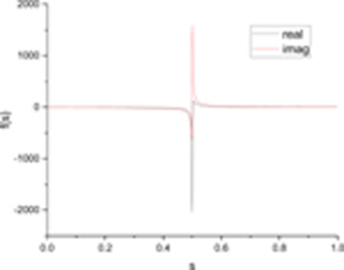
Figure 1: A partial fraction with Froissart doublets.

If the S-parameters of a circuit are acquired by FEM and interpolated by ARILM, often a smooth rational polynomial can be obtained. However, sometimes, the interpolated rational polynomial has a spike in the curve, given the term Froissart doublets. Froissart doublets are mainly owing to the numerical errors of the S-parameters at the sampling frequencies. Let’s explain the cause of the Froissart doublets with a simple partial fraction as:

$$f\left(s\right)=\frac{1.0+j2.0}{s-(0.5+j0.001)},0\le s\le 1,$$

(8)

which has a pole and a residual. Actually, the real part of the pole represents the normalized resonant frequency, while the imaginary part indicates the power loss of the corresponding circuit. If the imaginary part of the pole is very small, the circuit is close to lossless, and there will be a resonance, which is characterized by a spike in the curve as in Fig. 1.

This partial fraction expression has an advantage over the barycentric rational polynomial in that it indicates the location of the spike. Therefore, the latter will be converted into the sum of the former. Then, the residual and pole of every partial fraction term will be analyzed to find the connection among the spike, the poles, and the residuals.

B. Convert the Loewner interpolation into the partial fraction expression

Loewner interpolation can be rewritten as:

$$f_L\left(s\right)={\mathrm{\Sigma }}_{i=1}^p\frac{{\alpha }_i{w}_i}{s-{\lambda }_i}/{\mathrm{\Sigma }}_{i=1}^p\frac{{\alpha }_i}{s-{\lambda }_i}\triangleq N/D.$$

(9)

The zeros of $N$ are also the zeros of $f_L\left(s\right)$, while the zeros of $D$ are the poles of $f_L\left(s\right)$. The zeros of $D$ can be obtained by solving the following equation:

$$D={\mathrm{\Sigma }}_{i=1}^p\frac{{\alpha }_i}{s-{\lambda }_i}=0.$$

(10)

This equation is equivalent to a generalized eigenvalue problem:

$$\left[\begin{array}{ccccc}\hfill 0\hfill & \hfill {\alpha }_1\hfill & \hfill {\alpha }_2\hfill & \hfill \mathrm{\cdots }\hfill & \hfill {\alpha }_{\mathrm{p}}\hfill \\ \hfill 1\hfill & \hfill {\lambda }_1\hfill & & & \\ \hfill 1\hfill & & \hfill {\lambda }_2\hfill & & \\ \hfill \mathrm{⋮}\hfill & & & \hfill \mathrm{\ddots }\hfill & \\ \hfill 1\hfill & & & & \hfill {\lambda }_{\mathrm{p}}\hfill \end{array}\right]\left[\begin{array}{c}\hfill x_0\hfill \\ \hfill x_1\hfill \\ \hfill x_2\hfill \\ \hfill \mathrm{⋮}\hfill \\ \hfill x_{p+1}\hfill \end{array}\right]=$$

$$\lambda \left[\begin{array}{ccccc}\hfill 0\hfill & & & & \\ & \hfill 1\hfill & & & \\ & & \hfill 1\hfill & & \\ & & & \hfill \mathrm{\ddots }\hfill & \\ & & & & \hfill 1\hfill \end{array}\right]\left[\begin{array}{c}\hfill x_0\hfill \\ \hfill x_1\hfill \\ \hfill x_2\hfill \\ \hfill \mathrm{⋮}\hfill \\ \hfill x_{p+1}\hfill \end{array}\right],$$

(11)

which can be solved readily. Similarly, the zeros of $N$ can be attained by solving another generalized eigenvalue problem:

$$\left[\begin{array}{ccccc}\hfill 0\hfill & \hfill {\alpha }_1{w}_1\hfill & \hfill {\alpha }_2{w}_2\hfill & \hfill \mathrm{\cdots }\hfill & \hfill {\alpha }_{\mathrm{p}}{w}_{\mathrm{p}}\hfill \\ \hfill 1\hfill & \hfill {\lambda }_1\hfill & & & \\ \hfill 1\hfill & & \hfill {\lambda }_2\hfill & & \\ \hfill \mathrm{⋮}\hfill & & & \hfill \mathrm{\ddots }\hfill & \\ \hfill 1\hfill & & & & \hfill {\lambda }_{\mathrm{p}}\hfill \end{array}\right]\left[\begin{array}{c}\hfill x_0\hfill \\ \hfill x_1\hfill \\ \hfill x_2\hfill \\ \hfill \mathrm{⋮}\hfill \\ \hfill x_{\mathrm{p}+1}\hfill \end{array}\right]=$$

$$\lambda \left[\begin{array}{ccccc}\hfill 0\hfill & & & & \\ & \hfill 1\hfill & & & \\ & & \hfill 1\hfill & & \\ & & & \hfill \mathrm{\ddots }\hfill & \\ & & & & \hfill 1\hfill \end{array}\right]\left[\begin{array}{c}\hfill x_0\hfill \\ \hfill x_1\hfill \\ \hfill x_2\hfill \\ \hfill \mathrm{⋮}\hfill \\ \hfill x_{\mathrm{p}+1}\hfill \end{array}\right].$$

(12)

Once all the poles and residuals are obtained, formula (9) can be converted into the pole-zero expression:

$$f_L\left(s\right)=N/D=d{\mathrm{\Pi }}_{i=1}^{p-1}(s-c_i)/{\mathrm{\Pi }}_{i=1}^{p-1}(s-b_i).$$

(13)

The constant $d$ can be determined by any one of the sampling points, say $({\lambda }_1,w_1)$, as:

$$d=w_1{\mathrm{\Pi }}_{i=1}^{p-1}({\lambda }_1-b_i)/{\mathrm{\Pi }}_{i=1}^{p-1}({\lambda }_1-a_i).$$

(14)

Then, the pole-zero expression is rewritten as the sum of partial fractions:

$$d{\mathrm{\Pi }}_{i=1}^{p-1}(s-c_i)/{\mathrm{\Pi }}_{i=1}^{p-1}(s-b_i)={\mathrm{\Sigma }}_{i=1}^{p-1}\frac{a_i}{s-b_i}+a_0,$$

(15)

where both sides have the identical poles and only the residuals $a_i$ remain unknown. Since the partial fraction expression goes through the sampling points in (2), we have:

$$\left[\begin{array}{ccccc}\hfill 1\hfill & \hfill \frac{1}{{\lambda }_1-b_1}\hfill & \hfill \frac{1}{{\lambda }_1-b_2}\hfill & \hfill \mathrm{\cdots }\hfill & \hfill \frac{1}{{\lambda }_1-b_{\mathrm{p}-1}}\hfill \\ \hfill 1\hfill & \hfill \frac{1}{{\lambda }_2-b_1}\hfill & \hfill \frac{1}{{\lambda }_2-b_2}\hfill & \hfill \mathrm{\cdots }\hfill & \hfill \frac{1}{{\lambda }_2-b_{\mathrm{p}-1}}\hfill \\ & & & & \\ \hfill \mathrm{⋮}\hfill & & & \hfill \mathrm{\ddots }\hfill & \\ \hfill 1\hfill & \hfill \frac{1}{{\lambda }_{\mathrm{p}-1}-b_1}\hfill & \hfill \frac{1}{{\lambda }_{\mathrm{p}-1}-b_2}\hfill & & \hfill \frac{1}{{\lambda }_{\mathrm{p}-1}-b_{\mathrm{p}-1}}\hfill \end{array}\right]\left[\begin{array}{c}\hfill a_0\hfill \\ \hfill a_1\hfill \\ \hfill a_2\hfill \\ \hfill \mathrm{⋮}\hfill \\ \hfill a_{\mathrm{p}-1}\hfill \end{array}\right]=\left[\begin{array}{c}\hfill w_1\hfill \\ \hfill w_2\hfill \\ \hfill w_3\hfill \\ \hfill \mathrm{⋮}\hfill \\ \hfill w_p\hfill \end{array}\right].$$

(16)

Finally, the residuals $a_i$ are attained, and the barycentric rational polynomial (4) is converted into the partial fraction expression:

$$f_L\left(s\right)={\mathrm{\Sigma }}_{i=1}^p\frac{{\alpha }_i{w}_i}{s-{\lambda }_i}/{\mathrm{\Sigma }}_{i=1}^p\frac{{\alpha }_i}{s-{\lambda }_i}={\mathrm{\Sigma }}_{i=1}^{p-1}\frac{a_i}{s-b_i}+a_0.$$

(17)

C. Find and remove Froissart doublets

As discussed before, the Froissart doublets may be introduced by a partial fraction term, whose pole has a very small imaginary part. Therefore, we check every partial fraction term in (17) to determine which one may cause the doublets. As for the $k^{th}$ term, we divide (17) into two parts:

$$f_L\left(s\right)=\left[\frac{a_k}{s-b_k}\right]+\left[{\mathrm{\Sigma }}_{\begin{array}{c}\hfill i=1\hfill \\ \hfill i\ne k\hfill \end{array}}^{p-1}\frac{a_i}{s-b_i}+a_0\right]\triangleq f_k\left(s\right)+f_R\left(s\right),$$

(18)

where the poles are denoted by $b_i=b_{ix}+j{b}_{iy}$, and $\epsilon$ is a threshold to judge the doublets. If $b_{ky}={min}_{i=1,\mathrm{\cdots },p-1}(|b_{iy}|)$ and $|f_k\left(b_{kx}\right)|>|f_R\left(b_{kx}\right)|\times \epsilon$, there are doublets located at $b_{kx}$.

In order to remove the doublets, we delete the $k^{th}$ term in the partial fraction expression. In other words, $f_L\left(s\right)$ is approximated by $f_R\left(s\right)$. And then, the original sampling points are replaced with those computed by $f_R\left(s\right)$:

$$f_R\left(s_i\right)=f_i^{*},(i=1,2,3,\mathrm{\cdots },2p-1).$$

(19)

Finally, we construct another Loewner interpolation with these $(2p-1)$ new sampling points:

$$f_L^{*}\left(s\right)={\mathrm{\Sigma }}_{i=1}^p\frac{{\alpha }_i^{*}{w}_i^{*}}{s-{\lambda }_i}/{\mathrm{\Sigma }}_{i=1}^p\frac{{\alpha }_i^{*}}{s-{\lambda }_i},$$

(20)

which will be smooth and have no Froissart doublets.

IV. NUMERICAL RESULTS

Figure 2 shows a passive circuit with 26 ports, which is simulated by FEM to obtain the S-parameters over a very wide frequency band from 0.1 GHz to 250 GHz. We use ARILM to accomplish the wide band frequency sweeping, which starts with 3 sampling points and converges with 21 points. Note that all the S-parameters are interpolated with the same 21 frequencies. In order to determine the doublets, we set the threshold $\epsilon =1.0$.

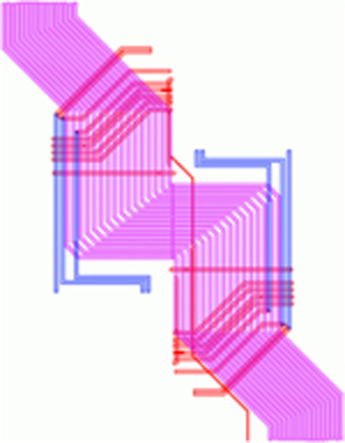
Figure 2: The 26-port passive circuit being simulated.

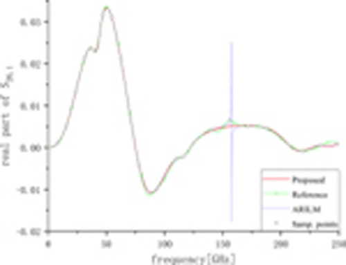
Figure 3: Real parts of $S_{26,1}$.

The curve of $S_{26,1}$is shown in Figs. 3 and 4. The interpolated rational polynomial has a spike at 157.6 GHz. Table 1 shows that the third partial fraction satisfies $b_{3y}={min}_{i=1,\mathrm{\cdots },p-1}(|b_{iy}|)$ and $|f_3\left(b_{3x}\right)|>|f_R\left(b_{3x}\right)|\times \epsilon$, where $b_{3x}=0.6305$ corresponds to 157.6 GHz. Therefore, the third partial fraction causes the spike. Figures 3 and 4 show that the Froissart doublets are removed by the proposed method and the resulting curves are still a good approximation to the reference curves.

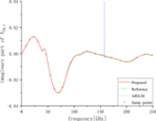
Figure 4: Imaginary parts of $S_{26,1}.$

Table 1: Residuals, poles, and function values of $S_{26,1}$

No.	Residual$a_i$	Pole$b_{ix}+j{b}_{iy}$	$f_k\left(b_{kx}\right)$	$f_R\left(b_{kx}\right)$
1	-0.000028 -j0.000008	0.952253 -j0.028919	0.000952 +j0.000272	0.000604 -j0.001296
2	-0.000315 +j0.000332	0.836766 +j0.076300	-0.004134 +j0.004345	0.004356 -j0.001552
3	-0.000008 -j0.000002	0.630471 -j0.000103	0.073629 +j0.021013	0.005099 -j0.001753
4	-0.000034 +j0.000076	0.463729 +j0.028439	0.001191 +j0.002662	0.000447 +j0.001365
5	-0.000724 +j0.003600	0.328455 +j0.099524	-0.007271 +j0.036169	0.027796 -j0.013676
6	0.000019 +j0.000014	0.326027 -j0.072588	-0.000260 -j0.000192	-0.008067 -j0.021470
7	0.000529 -j0.003231	-0.202759 +j0.057593	0.009192 -j0.056095	-0.006324 +j0.003122
8	0.003413 -j0.003550	0.157954 +j0.104093	0.032789 -j0.034107	-0.011102 -j0.030392
9	0.000085 +j0.000278	0.168986 +j0.022184	0.003820 +j0.012519	0.036364 -j0.000254
10	0.000197 -j0.000179	0.087280 +j0.053472	0.003678 -j0.003353	0.008093 +j0.009259

The curves of $S_{25,10}$are shown in Figs. 5 and 6. The interpolated rational polynomial has a spike at 33.32 GHz. As is shown in Table 2, this spike is generated by the ninth partial fraction, in which $b_{9x}=0.1329$ corresponds to 33.32 GHz. Figures 5 and 6 show that after removing the spike, the curves obtained by the proposed method are in good agreement with the reference curves.

The curves of S${}_{26}$${}_{,}$${}_2$${}_0$ are given in Fig. 7, which has no spike. Table 3 shows that the fifth partial fraction has the minimum imaginary part, but $|f_5\left(b_{5x}\right)|>|f_R\left(b_{5x}\right)|\times \epsilon$ is not satisfied. Therefore, the above three S-parameters validate the efficacy of the proposed method, which can exactly identify the partial fraction with Froissart doublets.

Figure 5: Real parts of $S_{25,10}$.

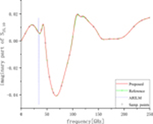
Figure 6: Imaginary parts of $S_{25,10}$.

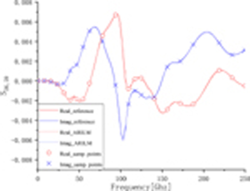
Figure 7: Real parts and imaginary parts of $S_{26,20}$.

Table 2: Residuals, poles, and function values of $S_{25,10}$

No.	Residue	Pole	$f_k\left(b_{kx}\right)$	$f_R\left(b_{kx}\right)$
1	-0.002966 -j0.001250	1.275554 -j0.013567	0.218629 +j0.092157	0.004306 +j0.009232
2	-0.000735 +j0.001602	0.834878 +j0.125776	-0.005848 +j0.012736	0.010899 +j0.011212
3	-0.000254 -j0.000258	0.609035 +j0.048807	-0.005195 -j0.005294	0.005349 +j0.008287
4	0.000137 +j0.000162	0.476290 +j0.032733	0.004186 +j0.004946	0.000630 +j0.015302
5	0.000615 +j0.000448	0.419796 +j0.033937	0.018121 +j0.013208	-0.013543 -j0.001148
6	-0.005674 +j0.003293	0.285817 +j0.111489	-0.050893 +j0.029541	0.026137 +j0.010261
7	0.000603 +j0.000059	0.172140 +j0.021737	0.027729 +j0.002702	0.034888 -j0.015548
8	0.003731 +j0.000644	0.088112 +j0.103326	0.036113 +j0.006236	0.018777 -j0.024063
9	-0.000004 -j0.000003	0.132949 +j0.000041	-0.086857 -j0.076599	0.020033 +j0.005948
10	0.000183 -j0.000006	-0.051439 -j0.058124	-0.003142 +j0.000098	0.000234 -j0.003244

Table 3: Residuals, poles, and function values of $S_{26,20}$

No.	Residue	Pole	$f_k\left(b_{kx}\right)$	$f_R\left(b_{kx}\right)$
1	-0.004838 -j0.008596	-1.362713 -j0.246348	0.019640 +j0.034892	0.004869 +j0.007194
2	-0.000198 -j0.000400	0.887203 +j0.102572	-0.001928 -j0.003898	-0.002806 +j0.005414
3	-0.001274 +j0.000307	0.672367 +j0.132489	-0.009615 +j0.002316	0.000149 +j0.011496
4	0.000217 +j0.000564	0.605122 +j0.075424	0.002880 +j0.007479	0.004231 -j0.002434
5	0.000005 +j0.000005	0.534310 +j0.013026	0.000364 +j0.000349	-0.000469 -j0.001958
6	-0.000191 +j 0.000034	0.412166 +j0.025577	-0.007484 +j0.001314	0.003694 +j0.001489
7	0.000023 -j0.000019	0.295191 +j0.029625	0.000788 -j0.000634	0.002878 +j0.004267
8	0.000300 +j0.000497	0.224718 +j0.088547	0.003387 +j0.005611	0.003941 +j0.000424
9	0.000023 -j0.000010	0.166183 +j0.020046	0.001129 -j0.000508	-0.002189 +j0.000268
10	0.000003 -j0.000053	0.091299 +j0.063231	0.000045 -j0.000837	-0.001142 -j0.000366

V. CONCLUSION

This paper proposes a new technique to remove the Froissart doublets in an adaptive rational interpolation based on the Loewner matrix. Numerical results indicate the efficacy of the proposed method. Although the proposed technique is tailored for ARILM, it is also applicable to other rational interpolations. In addition, the threshold $\epsilon$ is manually set according to specific circuits, and it will be chosen automatically in future.

ACKNOWLEDGMENT

This work is supported partially by the Natural Science Basic Research Program of Shaanxi Province (Program No. 2021JM-129).

REFERENCES

[1] A. Karwowski, A. Noga, and T. Topa, “Computationally efficient technique for wide-band analysis of grid-like spatial shields for protection against LEMP effects,” Applied Computational Electromagnetics Society (ACES) Journal, vol. 32, no. 1, pp. 87-92, 2017.

[2] Y. Zhang, D. Huang, and J. Chen, “Combination of asymptotic phase basis functions and matrix interpolation method for fast analysis of monostatic RCS,” Applied Computational Electromagnetics Society (ACES) Journal, vol. 28, no. 1, pp. 49-56, 2013.

[3] S. M. Seo, C. Wang, and J. Lee, “Analyzing PEC scattering structure using an IE-FFT algorithm,” Applied Computational Electromagnetics Society (ACES) Journal, vol. 24, no. 2, pp. 116-128,2009.

[4] D. Schobert and T. Eibert, “Direct field and mixed potential integral equation solutions by fast Fourier transform accelerated multilevel Green’s function interpolation for conducting and impedance boundary objects,” Applied Computational Electromagnetics Society (ACES) Journal, vol. 26, no. 12, pp. 1016-1023, 2011.

[5] F. S. de Adana, O. Gutiérrez, L. Lozano, and M. F. Cátedra, “A new iterative method to compute the higher order contributions to the scattered field by complex structures,” Applied Computational Electromagnetics Society (ACES) Journal, vol. 21, no. 2, pp. 115-125, 2006.

[6] Y. Zhang, Z. Wang, F. Zhang, X. Chen, J. Miao, and W. Fan, “Phased array calibration based on measured complex signals in a compact multiprobe setup,” IEEE Antennas and Wireless Propagation Letters, vol. 21, no. 4, pp. 833-837, 2022.

[7] Z. Liu, R. Chen, D. Ding, and L. He, “GTD model based cubic spline interpolation method for wide-band frequency- and angular- sweep,” Applied Computational Electromagnetics Society (ACES) Journal, vol. 26, no. 8, pp. 696-704,2011.

[8] B. Gustavsen and A. Semlyen, “Rational approximation of frequency domain responses by vector fitting,” IEEE Transactions on Power Delivery, vol. 14, no. 3, pp. 1052-1061, Jul. 1999.

[9] G. A. Baker, J. L. Gammel, and J. G. Wills, “An investigation of the Padé approximant method,” Journal of Mathematical Analysis & Applications, vol. 2, no. 1, pp. 405-418, 1961.

[10] B. Essakhi and L. Pichon, “An efficient broadband analysis of an antenna via 3D FEM and Padé approximation in the frequency domain,” Applied Computational Electromagnetics Society (ACES) Journal, vol. 2, no. 1, pp. 143-148, 2006.

[11] A. C. Antoulas, J. A. Ball, J. Kang, and J. C. Willems, “On the solution of the minimal rational interpolation problem,” Linear Algebra and its Applications, vol. 137-138, no. 4805, pp. 511-573, 1990.

[12] H. Yuan, W. Bao, C. Lee, B. F. Zinser, S. Campione, and J. Lee, “A method of moments wide band adaptive rational interpolation method for high-quality factor resonant cavities,” IEEE Transactions on Antennas and Propagation, vol. 70, no. 5, pp. 3595-3604, May, 2022.

[13] B. Beckermann, G. Labahn, and A. C. Matos, “On rational functions without Froissart doublets,” Numerische Mathematik, vol. 138, pp. 615-633, 2018.

[14] P. Gonnet, S. Guttel, and L. N. Trefethen, “Robust Padé approximation via SVD,” SIAM Review, vol. 55, pp. 101-117, Mar. 2013.

[15] J. Gilewicz and Y. Kryakin, “Froissart doublets in Padé approximation in the case of polynomial noise,” Journal of Computational and Applied Mathematics, no. 153, pp. 235-242.

[16] R. P. Brent, F. G. Gustavson, and D. Y. Y. Yun, “Fast solution of Toeplitz systems of equations and computation of Padé approximants,” Journal of Algorithms, vol. 1, pp. 259–295, 1980.

[17] D. Belkić and K. Belkić, “Padé–Froissart exact signal-noise separation in nuclear magnetic resonance spectroscopy,” Journal of Physics B, vol. 44, pp. 1-19, 2011.

[18] D. Bessis, “Padé approximations in noise filtering,” Journal of Computational and Applied Mathematics, vol. 66, pp. 85–88, 1996.

[19] Y. Nakatsukasa, O. Sète, and L. N. Trefethen, “The AAA algorithm for rational approximation,” SIAM Journal on Scientific Computing, vol. 40, no. 3, pp. A1494-A1522, 2018.

[20] J. Gilewicz and M. Pindor, “Padé approximants and noise: A case of geometric series,” Journal of Computational and Applied Mathematics, vol. 87, pp. 199-214, 1997.

[21] J. Gilewicz and M. Pindor, “Padé approximants and noise: Rational functions,” Journal of Computational and Applied Mathematics, vol. 105, no. 1, pp. 285-297, 1999.

BIOGRAPHIES

Haobo Yuan was born in Tianmen, Hubei, China, in 1980. He received his B.S., M.S., and Ph.D. degrees in Electromagnetic Fields and Microwave Technology from Xidian University, Xi’an, China, in 2003, 2006, and 2009, respectively. Since 2006, he has been with the School of Electronic Engineering, Xidian University, where he is an Associate Professor. He was a post doctoral researcher at Ohio State University in 2019. His current research interests include computational electromagnetics, antenna measurements, and electromagnetic compatibility.

Jungang Ren was born in Xi’an, Shaanxi, China, in 1998. He received his B.Eng. degree in Electronic Information Engineering from Xidian University, Xi’an, China, in 2020. He is currently working towards an M.S. degree with Xidian University. His research interests are numerical techniques in computational electromagnetics.

Yujie Li received her B.Eng. degree in Electronic Information Engineering from the North University of China, Taiyuan, China in 2017. She is currently pursuing an M.Eng. degree with Xidian University. Her research interests are antenna measurement techniques and numerical methods in computational electromagnetics.

Xiaoming Huang received his B.Eng. degree in Electrical Engineering from Zhengzhou University, Henan, China, in 2021. He is currently pursuing an M.S. degree with Xidian University, Xi’an. His research interests are the numerical techniques in computational electromagnetics.

ACES JOURNAL, Vol. 38, No. 1, 60–66
doi: 10.13052/2023.ACES.J.380109
© 2023 River Publishers

ABSTRACT

I. INTRODUCTION

II. RATIONAL INTERPOLATION BASED ON LOEWNER MATRIX

III. REMOVING FROISSART DOUBLETS IN RATIONAL INTERPOLATION

A. Observe the Froissart doublets

B. Convert the Loewner interpolation into the partial fraction expression

C. Find and remove Froissart doublets

IV. NUMERICAL RESULTS

V. CONCLUSION

ACKNOWLEDGMENT

REFERENCES

BIOGRAPHIES