Application of Artificial Neural Network Base Enhanced MLP Model for Scattering Parameter Prediction of Dual-band Helical Antenna

Ahmet Uluslu

Department of Electronics and Automation
Istanbul University-Cerrahpaşa, Istanbul, 34500, Turkey
auluslu@iuc.edu.tr

Submitted On: June 23, 2022; Accepted On: June 10, 2023

ABSTRACT

Many design optimization problems have problems that seek fast, efficient and reliable based solutions. In such cases, artificial intelligence-based modeling is used to solve costly and complex problems. This study is based on the modeling of a multiband helical antenna using the Latin hypercube sampling (LHS) method using a reduced data enhanced multilayer perceptron (eMLP). The proposed helical antenna is dual-band and has resonance frequencies of 2.4 GHz and 2.75 GHz. The enhanced structure of the artificial neural network (ANN) was tested using 4 different training algorithms and a maximum of 10 different MLP architectures to determine the most suitable model in a simple and quick way. Then, performance comparison with other ANN networks was made to confirm the success of the model. Considering the high cost of antenna simulations, it is clear that the proposed model will save a lot of time. In addition, thanks to the selected sampling model, a wide range of modeling can be done with minimum data. When the target and prediction data are compared, it is seen that these data overlap to a large extent. As a result of the study, it was seen that the ANN modeling and the 125 samples used, were as accurate as an electromagnetic (EM) simulator for other input parameters in a wide range selected.

Index Terms: ANN, design modeling, dual-band, enhanced algorithm, helical antenna.

I. INTRODUCTION

An antenna is the name given to a metal device or converter manufactured to receive radio waves [1]. There are many types such as dipole, monopole, microstrip, satellite, periodic and array antenna. Helical antennas consist of a coil with a constant pitch of turns placed on a cylindrical surface, fed by a special cable and connected to a conductive plane [2]. A result of this structure is that the antenna size can decrease. Today, mobile stations count for a large share among the places where helical antennas are widely used. The performance of the mobile station is directly dependent on the performance of the helical antenna. Helical antennas are often preferred in portable devices such as mobile phones because they occupy less space and have broadband. The helical antenna, originally designed by Kraus, was used to detect radiation [3]. Due to its broadband advantage, it has also been popular in satellite systems for a while. Helical antennas are available in various designs according to their usage areas [4–7]. In addition, studies on underwater communication are substantial [8–10]. Just like in mobile phones, 2.4 GHz radio frequency is used in underwater applications [11–13]. In recent years, artificial intelligence (AI) algorithms have been used in many high-performance circuit designs. They have been frequently used in many different microwave circuit designs [14], such as unit cell models [15–16] for large-scale reflective array antenna designs and modeling of microstrip transmission lines [17–18]. In a few recent studies, there are AI-based models of antennas [19–20]. The first of these studies was carried out for the capacitive feed antenna [19]. The total number of samples in the study is 51,300. In the other study, modeling of microstrip antenna was discussed [20]. However, in this study, basing the gap width and number of steps on user preference increased the total number of samples used, causing it to be 18,450. Normally, the desired features of antenna design are obtained by experimentation. However, this method is quite costly when the antenna simulation time is taken into account. In the study, the solution of the design optimization problem of a dual-band helical antenna with an elliptical geometric structure, which has pioneered many design problems, is proposed using a fast, efficient, accurate and reliable based model with a low cost. MATLAB 2021a program was used for antenna electromagnetic (EM) simulations. An artificial neural network (ANN) model is designed to predict the variation of the S $_{11}$ (dB) parameter of a helical antenna with resonance frequencies of 2.4 GHz and 2.75 GHz along the frequency band determined indifferent sizes.

In section II of the study, the parameters for the design of the helical antenna will be analyzed. In section III the data reduction with the Latin hypercube sampling (LHS) method and the details of the proposed network model will be discussed. In section IV the results of the study will be presented and the performance comparison with different ANN networks will be given. In section V, the paper will be concluded with evaluations and suggestions on the overall study.

II. DESIGN PROCESS OF HELICAL ANTENNA

Helical antennas have a circular polarization feature preferred in broadband VHF and UHF bands. In short, it can be defined as the practical configuration of the EM radiator. It consists of a coil of pipe or a thick copper wire wound like the thread of a screw. Most of the time the helix is resting on a base as shown in Fig. 1. The parameters used to define the helical antenna geometry are given in Table 1 along with their definitions and design used values.

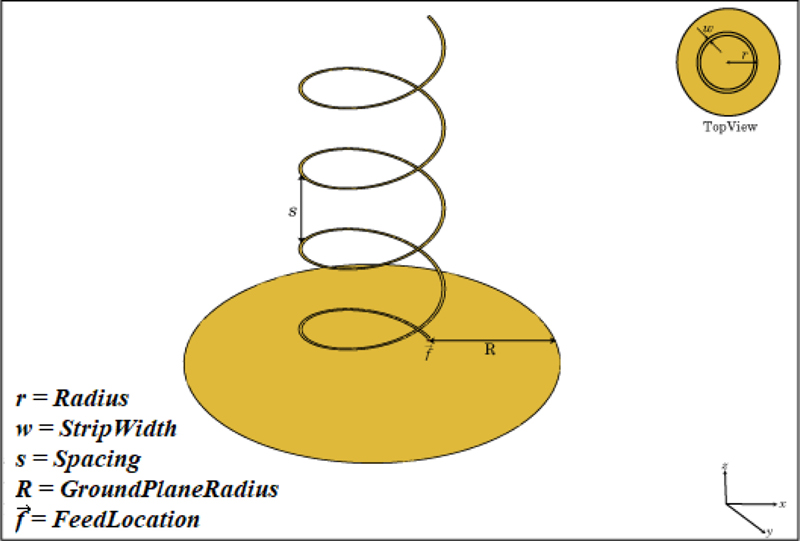
Figure 1: Physical parameters of helical antenna.

Table 1: Helix design parameters

Parameter	Value	Definition
Radius	-	Radius of turns
Width	-	Strip width
Turns	-	Number of turns of helix
Spacing	35 (mm)	Spacing between turns
Winding Direction	CW	Direction of helix turns (windings)
Ground Plane Radius	75 (mm)	Ground plane radius
Feed Stub Height	1.0000e-03 (m)	Feeding stub height from ground
Conductor	PEC	Type of metal material

III. PROPOSED METHOD

A. Dataset reduction using the Latin hypercube sampling method

ANNs can be trained due to their structure. They keep the data obtained during training as the connection weight between nerve cells. This process can also be defined as the determination of connection weights. These weights store the information that will be needed during the calculation of the test data of the network [21]. It is ensured that the training cost is very low in order for the network to determine the most optimal connection weights. Here, the low rate of error in the test result is directly proportional to the training error. Therefore, the training error should be kept low as a priority. Here, the data set selection is of great importance. Input parameter ranges to be used to determine the optimum results of the network in the desired frequency band range have been determined based on the optimization study carried out in the case studies [22–23]. In these studies, the design of the helical antenna with optimization algorithms was discussed [22–23]. However, as it is well known, optimization processes are both costly and long-term processes. Therefore, in many studies, the modeling process with the optimum data set gives results in a short time as well as its low cost. Here, data reduction is among the methods frequently used in such applications to further reduce the cost. For this reason, using a sampling technique called LHS, the widest range of data set was extracted. LHS is a popular stratified sampling technique first proposed by MacKay [24] and further developed by Iman and Conover [25]. It is a sampling method of random designs that try to be evenly distributed in the design space. With the LHS, one must first decide how many sample points to use, and remember in which row and column the sample point is taken for each sample point. This configuration is similar to having N rooks on a chessboard without threatening each other [24–25]. Training models in deep learning can be divided into 3 classes in general. These are named as underfit model, overfit model and good fit model. Of these, the overfit model that learns the training dataset very well, performs well in the training dataset, but cannot perform well in the test sample. This common overfitting issue was overcome by choosing theLHS model.

Here, 3 different design parameters of a dual band helical antenna are extracted in the intervals and number of samples indicated in Table 2. In addition, a total of 100 frequency samples with equal step spacing in the 1.5-3.5 GHz band range were selected. All these processes were performed by a computer with 8th generation Intel Core i7 CPU, 3.20 GHz processor and8 GB RAM.

Table 2: Test and training data sets

Parameter	Range	Sampling Method	Number of Samples
Radius (r) (mm)	20–30	Latin hypercube	5
Width (w) (mm)	1– 4	Latin hypercube	5
Turns (t)	1– 4	Latin hypercube	5
Frequency (GHz)	1.5–3.5	Linear	100
Total Sample (number of samples X frequency)	-	-	125x100

B. eMLP model

ANNs are frequently encountered in design problems because of their successful performance. Multilayer perceptron (MLP) neural network is one of the most popular among ANNs. The choice of training algorithm type (trainlm, trainbr etc. [27–30]) and architecture (number of hidden layers and neurons) used in the problems solved using this network model is one of the most important points. It is very difficult to predict which of these choices will be closer to the target. There are various studies on this subject [31–35]. A new trained constructive model has been proposed to obtain the minimum mean error value with optimum cost by training ANNs [36]. Here, this suggestion is further developed, using a small number of models and a certain number of hidden layers and neurons. In the study, mean error values are recorded throughout the learning process. When this value does not catch a new decrease during the training period, it is concluded that the network has reached saturation. At the same time, other architectural results are recorded and the threshold value is determined. According to this threshold value, the model determines how many MLP architectures it will create in total for each training algorithm. In addition, the maximum value for the architecture experiment is determined by the user. For each architecture, the number of hidden layers and neurons is automatically adjusted according to the average error value of the algorithm. This enhanced multilayer perceptron (eMLP) model provides great convenience for the user compared to the standard architecture [31–32], [36–37].

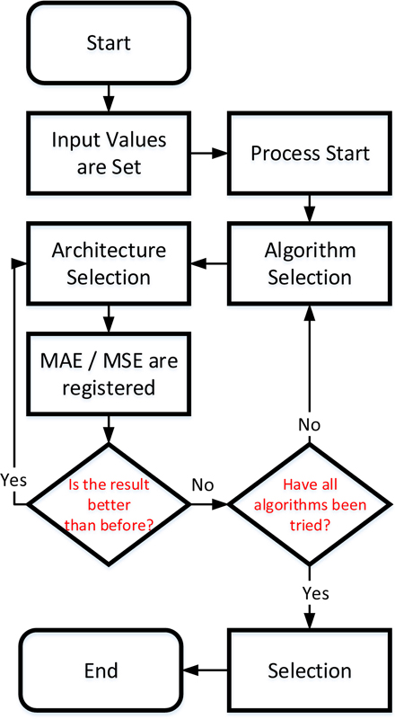
Figure 2: Flow chart of the modeling process for eMLP.

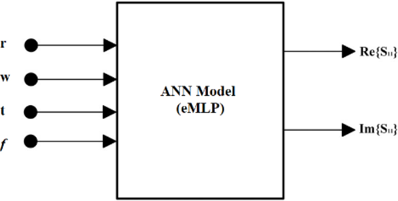
Figure 3: ANN model for training the S $_{11}$ (dB) parameter of the helical antenna.

In this designed eMLP model, first the model parameters are set. These are the training algorithm types to be used: trainbr, trainlm etc. [26–30]. MLP architecture consists of parameters such as the number of hidden layers, the number of neurons to be used in the hidden layers, and the maximum number of architectural trials. In the next process, the modeling process is started for the determined training algorithms and architectures.

Mean absolute error (MAE)/Mean squared error (MSE)’s generated as a result of each modeling process are recorded. The system compares the MSE ratio with the previous result and decides whether to continue with the new architecture. In short, it is expected to reach saturation. This process is repeated separately for each training algorithm set at the beginning. As a result of all these processes, the training algorithm/architecture with the minimum MSE is accepted as the best model. All these steps are presented in Fig. 2 as a flow chart. In addition, the black box model of the ANN is shown in Fig. 3.

MSE and MAE can be counted among the main performance indicators used in the performance evaluations of ANN and machine learning (ML) methods [20], [35]. MSE gives an absolute number of how much the predicted results differ from the actual number. Not much insight can be interpreted from a single result, but it gives a real number to compare with other model results and helps with the choice of the best regression model. The MAE sums the absolute error value, a more direct representation of the sum of the error terms. It is more suitable for comparing the results of other studies with or without normalization. In the study, both performance evaluation results are given as a table.

For the proposed model for each mean error value the training depends on two parameters: algorithm type and architecture (hidden layer counts and neuron counts). The purpose of this model is to find the result with the best mean error simply and quickly.

IV. CASE STUDY

The study consists of three main parts. The first stage includes the study results for the training algorithms/architectures determined for the proposed eMLP model. Here, the most successful training algorithm/architecture is determined, and the second step is to compare the performance of the proposed model with other ANN models. As a final step, in order to reveal that the study is applicable in real life, a design was made with a selected model using the 3D EM simulation tool CST program.

A. Experimental work for eMLP

In this part of the study, a multi-band helical antenna design with 3 different design parameters based on eMLP, and modeling in the 1.5-3.5 GHz band will be studied. The proposed antenna has dual bands with resonance frequencies of 2.4 GHz and 2.75 GHz. Based on the helical antenna ANN model in Fig. 2, there are 3 input variables that will directly affect the output parameter S $_{11}$ (dB). When frequency is added to these, there are a total of 4 input parameters specified in Table 2. In the study, firstly, the ranges for the design parameters are determined. Then, the input data set is created with the LHS method. S $_{11}$ results for the selected input data set are determined with the help of an EM simulator. By combining all these data, half of the input/output data set is separated as training data and the other half as test data, and the modeling process is started using eMLP. As a result of all these operations, the model with the minimum average error is considered the optimal result. All this is presented as a flowchart in Fig. 4.

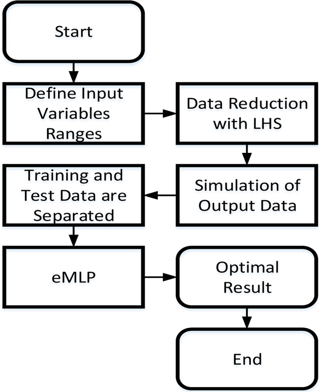
Figure 4: Flow chart of modeling process of LHS and eMLP based helical antenna.

Table 3: General comparison of MAE and MSE based eMLP models

Training Algorithm	Architecture	Train Error (MSE)	Test Error (MSE)	Train Error (MAE)	Test Error (MAE)	Time (sec.)
trainbr	5 10	6.08	7.77	1.37	1.40	11.2
	10 15	6.08	7.77	1.37	1.40	21.7
	15 20	6.08	7.77	1.37	1.40	45.7
	5 10 15	0.12	97.6	0.24	0.66	26.7
	5 15 20	0.03	0.46	0.11	0.15	53.7
	10 15 20	0.02	1.34	0.09	0.18	72.4
	5 10 15 20	0.03	0.32	0.11	0.15	83.4
	10 10 15 20	0.02	0.21	0.09	0.13	101.7
	10 15 15 20	0.01	0.22	0.08	0.14	135.9
trainlm	5 10	0.69	1.18	0.51	0.55	9.6
	10 15	0.16	0.39	0.26	0.29	21.4
	15 20	0.03	0.22	0.12	0.16	41.5
	5 10 15	0.14	0.70	0.25	0.31	25.0
	5 10 15 20	0.02	0.44	0.09	0.16	47.2
	10 10 15 20	0.02	0.37	0.10	0.18	5.0
	10 15 15 20	0.01	0.84	0.08	0.16	13.9
trainrp	5 10	6.12	7.99	1.37	1.44	2.7
	10 15	6.05	7.76	1.36	1.38	3.4
	15 20	5.68	7.39	1.36	1.40	4.1
	5 10 15	6.00	7.68	1.35	1.38	4.0
	5 15 20	6.08	8.61	1.37	1.60	4.8
	10 15 20	2.80	4.10	0.91	0.96	5.2
trainscg	5 10	6.07	7.77	1.37	1.40	4.6
	10 15	6.06	7.77	1.37	1.41	6.0
	15 20	6.00	7.71	1.36	1.42	7.6
	5 10 15	6.07	7.77	1.37	1.40	7.3
	10 15 20	5.99	7.75	1.35	1.38	9.8
	5 10 15 20	6.08	7.78	1.37	1.40	11.2
	10 10 15 20	6.07	7.79	1.38	1.42	11.9
	10 15 15 20	3.02	5.15	0.97	1.16	12.9

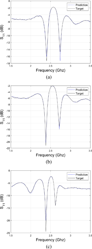
Figure 5: eMLP model performance parameter of return loss (S $_{11}$ ) for antenna: (a) r=27 (mm), w=1.5 (mm), t=2.6, (b) r=27 (mm), w=2 (mm), t=2.6, and (c) r=27 (mm), w=2.5 (mm), t=3.3.

The MSE and MAE values for the training and test, which are the result of the study performed in line with the steps given in order as the flow chart in Fig. 4, are given numerically in Table 3. According to the results indicated in Table 3, it is seen that the increase in the number of hidden layers and neurons in the architecture increases the modeling time. When we compare the training algorithms with the same architecture in terms of modeling time, it is seen that the fastest training algorithm is ‘trainrp’. However, in architecture, it is seen that increasing the number of hidden layers and neurons does not always cause a decrease in the error rate. This situation varies according to the selected training algorithm. In addition, the importance of the eMLP model in finding the optimal architecture is clearly seen. In the study, a maximum of 10 different MLP architecture experiments were made for 4 different training algorithms. Here, it is appropriate to select 10 as the maximum value, since the modeling is terminated before reaching 10 different trials for each training algorithm. As a result of the study, values with a lower error were obtained as a result of modeling with the ‘trainbr’ training algorithm. In the ‘trainbr’ training algorithm, which has the most successful results, it is seen that it has a 4 hidden layer MLP architecture with ‘10-10-15-20’ neurons. The results obtained as a result of this most successful model are given graphically in Figs. 5 (a), (b) and (c) as the variation of S $_{11}$ (dB) with frequency as target and prediction data. As can be seen from the graphics, a high success rate has beenachieved.

B. Performance comparison with other ANNmodels

Of course, these very low error rates obtained from the study do not directly confirm the success of the study. In order to support the success of the proposed model, performance comparisons were made with other widely used ANNs. Here, modeling studies were carried out with 3 different neural networks apart from eMLP. Since the radial basis (RB) model does not take any input parameters, it is used directly. In the radial basis function (RBF) and general regression neural network (GRNN) models, experiments were made for different spread parameters, and the result with the lowest error was selected. The most successful results obtained are graphically presented as the variation of S $_{11}$ (dB) with frequency in Figs. 6 (a), (b) and (c) for 4 different ANNs. In addition, error rates and time are given numerically in Table 4. As can be seen from the results, the closest results to the target line were obtained with the eMLP model. Although GRNN is lower in time cost, this situation can be ignored since it is in the order of seconds.

Table 4: Performance comparison of ANN models based on MEA/MSE

ANN	Train Error (MSE)	Test Error (MSE)	Train Error (MAE)	Test Error (MAE)	Time (sec.)
GRNN	1.16	1.77	0.67	0.70	94.2
RBE	1.80	3.85	0.79	1.00	168.7
RB	3.40	4.66	1.04	1.10	192.4
eMLP	0.02	0.21	0.09	0.13	101.7

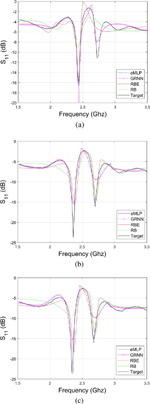
Figure 6: Comparison of different ANN model performance parameter of the return loss (S $_{11}$ ) of the antenna: (a) r=27 (mm), w=1 (mm), t=2.95, (b) r=27 (mm), w=2.5 (mm), t=2.6, and (c) r=27 (mm), w=3 (mm), t=2.60.

C. Simulation verification with 3D designprogram

One of the most successful results was selected and modeled in the 3D EM simulation tool CST microwave studio program. The results from the EM program show that the gain is 11.9 dB for 2.4 GHz and 9.81 dB for 2.75 GHz. Also, the far field gain for 2.4 GHz and 2.75 GHz is shown in Figs. 7 (a) and (b), respectively. The similarity of the simulation results revealed that this antenna is applicable to the real error. In addition, the antenna simulation time takes an average of 45-50 seconds for 1 sample. If it is calculated that the modeling process is done for 62 samples, this time is approximately 50 minutes. In the eMLP model, this process can be done in about 102 seconds.

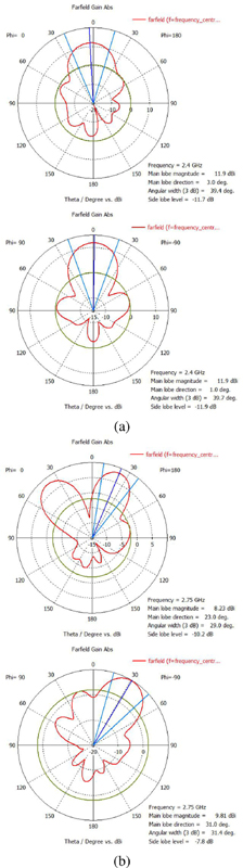
Figure 7: Farfield gain of helical antenna for (a) 2.4 GHz and (b) 2.75 GHz.

V. CONCLUSIONS

Here, a fast, accurate and reliable solution to the design problem, which is very costly for antenna designers, is provided by using the proposed eMLP model for multi-band helical antenna design. Return loss (S $_{11}$ ) of less than -10 dB was observed throughout the process at approximately 2.4 and 2.75 GHz resonance frequencies. Data reduction was made by using the LHS method in the selection of the data set. Thus, the total number of samples was kept to a minimum. Successful results were obtained with the proposed eMLP model using this data set. To confirm this success, performance comparisons of different ANN types were made. With this method, the very costly trial-and-error method, used in antenna design, is obsolete. In addition, instead of starting the design with a standard geometry, starting with optimized value ranges from a previous study enabled the problem to achieve clearer results. In addition, the design created in the CST program was used to compare the MATLAB results with another 3D EM simulation tool which revealed that it is applicable in real life. Therefore, as a result of the study, it has been seen that the proposed model is both more economical in terms of calculation and as accurate and safe as the EM simulator in the design of the dual band helical antenna. In addition, the proposed model is not limited to the helical antenna, the model can also be successfully applied to other design optimization problems by changing the network model.

REFERENCES

[1] C. A. Balanis, Antenna Theory: Analysis and Design, 3rd ed. New Jersey, John Wiley & Sons, 2005.

[2] Y. Liang, J. Zhang, Q. Liu, and X. Li, “High-power dual-branch helical antenna,” IEEE Antennas and Wireless Propagation Letters, vol. 17, no. 3, pp. 472-475, Mar. 2018

[3] J. D. Kraus, Antennas, 2nd ed. McGraw-Hill College, Mar. 1988.

[4] X. Tang and J. Zhang, “A strip-helical dipole antenna with wide bandwidth and high gain,” International Symposium on Antennas and Propagation (ISAP), Okinawa, Japan, pp. 82-83, Oct. 2016.

[5] S. I. H. Shah, S. Gosh, M. M. Tentzeris, and S. Lim, “A novel bio inspired pattern reconfigurable quasi-yagi helical antenna using origami DNA,” International Symposium on Antennas and Propagation (ISAP), Busan, Korea (South), pp. 1-2, Oct. 2018.

[6] S. H. Eedala, S. Elakiyaa, R. Nethra, R. Asha, and M. Jayakumar, “Design of helical array antenna based ground terminal for satellite communication on the move,” 4th International Conference on Electronics, Communication and Aerospace Technology (ICECA), Coimbatore, India, pp. 559-563, Nov. 2020.

[7] F. Hyjazie, W. Tong, and H. Boutayeb, “Multi/wide band printed quad helical antenna,” IEEE International Symposium on Antennas and Propagation and North American Radio Science Meeting, Montreal, QC, Canada, pp. 1893-1894, July 2020.

[8] M. Barbeau, J. Garcia-Alfaro, E. Kranakis, and S. Porretta, “The sound of communication in underwater,” Ad Hoc Networks, vol. 223, pp. 13-23, Jan. 2018.

[9] I. F. Akyildiz, D. Pompili, and T. Melodia, “Underwater acoustic sensor networks: Research challenges,” Hindawi, vol. 3, no. 3, pp. 257-279, May 2005.

[10] M. Subha and K. S. Divya, “Technologies used in underwater wireless communication,” International Journal of Innovative Research in Computer and Communication Engineering, vol. 5, no. 6, pp. 91-95, July 2017.

[11] A. N. Jaafar, H. Ja’afar, I. Pasya, Y. Yamada, R. Abdullah, M. A. Aris, and F. N. M. Redzwan, “Analysis of helical antenna for wireless application at 2.4 GHz,” IEEE Asia-Pacific Conference on Applied Electromagnetics (APACE), Melacca, Malaysia, pp. 1-5, Nov. 2019.

[12] N. Destria, M. Artiyasa, S. Gumilar, R. Azhari, A. Badrudin, M. A. Maulidan, and J. A. Pradiftha, “Design of 2.4 GHz helix antenna for increasing wifi signal strength using managal and wirelesmon application,” International Conference on Computing, Engineering, and Design (ICCED), Kuala Lumpur, Malaysia, pp. 1-5, Nov. 2017.

[13] M. Márton, Ľ. Ovseník, J. Turán, M. Špes, and J. Urbanský, “Comparison of helix antennas operated on 2.4, 5.2 and 9.2GHz for FSO/RF hybrid system,” 29th International Conference Radioelektronika, Pardubice, Czech Republic, pp. 1-4, Apr.2019.

[14] F. Güneş, P. Mahouti, S. Demirel, M. A. Belen, and A. Uluslu, “Cost-effective GRNN-based modeling of microwave transistors with a reduced number of measurements,” International Journal of Numerical Modelling: Electronic Networks, Devices and Fields, vol. 30, no. 3-4, Aug. 2017.

[15] F. Güneş, S. Demirel, and S. Nesil, “A novel design approach to X-band Minkowski reflectarray antennas using the full-wave EM simulation-based complete neural model with a hybrid GA-NM algorithm,” Radioengineering, vol. 23, no. 1, pp. 144-153, Apr. 2014.

[16] P. Mahouti, F. Gunes, A. Caliskan, and M. A. Belen, “A novel design of non-uniform reflectarrays with symbolic regression and its realization using 3-D printer,” Applied Computational Electromagnetics Society (ACES) Journal, vol. 34, no. 2, pp. 280-285, Feb. 2019.

[17] D. Krishna, J. Narayana, and D. Reddy, “ANN models for microstrip line synthesis and analysis,” World Academy of Science, Engineering and Technology, International Science Index 22, International Journal of Electrical, Computer, Energetic, Electronic and Communication Engineering, vol. 2, no. 10, pp. 2343-234, Oct. 2008.

[18] P. Mahouti, F. Güneş, M. A. Belen, and S. Demirel, “Symbolic regression for derivation of an accurate analytical formulation using ‘Big Data’ an application example,” Applied Computational Electromagnetics Society (ACES) Journal, vol. 32, no. 5, pp. 372-380, May 2017.

[19] N. Calik, M. A. Belen, and P. Mahouti, “Deep learning base modified MLP model for precise scattering parameter prediction of capacitive feed antenna,” International Journal of Numerical Modelling: Electronic Networks, Devices and Fields, vol. 33, no. 2, Sep. 2019.

[20] P. Mahouti, “Design optimization of a pattern reconfigurable microstrip antenna using differential evolution and 3D EM simulation-based neural network model,” International Journal of RF and Microwave Computer-Aided Engineering, vol. 29, no. 8, Aug. 2019.

[21] Z. Şen, Yapay Sinir Ağlar $ı$ İlkeleri, İstanbul, Su Vakfı Yayınları, 2004.

[22] M. Kalkancı and A. Günday, “Triangular bowtie antenna design and modelling,” Research & Reviews in Engineering, Gece Publishing, May 2021.

[23] N. Timürtaş, “Honey Bee Mating Optimization About to Design Antennas,” Y $ı$ ld $ı$ z Teknik Üniversitesi / Fen Bilimleri Enstitüsü / Elektronik ve Haberleşme Mühendisliği Ana Bilim Dal $ı$ / Haberleşme Bilim Dal $ı$ , Yıldız, 2018.

[24] M. MaKa, R. Beckman, and W. Conover, “A comparison of three methods for selecting values of input variables in the analysis of output from computer code,” Technimeterics, vol. 21, no. 1, pp. 239-245, May 1979.

[25] R. Iman and W. Conover, “Small sample sensitivity analysis techniques for computer models, with an application to risk assessment,” Communications in Statistics-Theory and Methods, vol. 9, no. 17, pp. 1749-1842, Jan. 1980.

[26] A. D. Anastasiadis, G. D. Magoulas, and M. N. Vrahatis, “New globally convergent training scheme based on the resilient propagation algorithm,” Neurocomputing, vol. 64, pp. 253-270, Mar. 2005.

[27] D. J. C. MacKay, “Bayesian interpolation,” Neural Computation, vol. 4, no. 3, pp. 415-447, May 1992.

[28] D. Pham and S. Sagiroglu, “Training multilayered perceptrons for pattern recognition: A comparative study of four training algorithms,” International Journal of Machine Tools and Manufacture, vol. 41, no. 3, pp. 419-430, Feb. 2001.

[29] S. Ali and K. A. Smith, “On learning algorithm selection for classification,” Applied Soft Computing, vol. 6, no. 2, pp. 119-138, Jan. 2006.

[30] F. D. Foresee and M. T. Hagan, “Gauss-Newton approximation to Bayesian learning,” Proceedings of International Conference on Neural Networks (ICNN’97), Houston, TX, USA, pp. 1930-1935, June 1997.

[31] N. Çalik, M. A. Belen, P. Mahouti, and S. Koziel, “Accurate modeling of frequency selective surfaces using fully-connected regression model with automated architecture determination and parameter selection based on bayesian optimization,” IEEE Access, vol. 9, pp. 38396-38410, 2021.

[32] S. Masmoudi, M. Frikha, M. Chtourou, and A. B. Hamida, “Efficient mlp constructive training algorithm using a neuron recruiting approach for isolated word recognition system,” International Journal of Speech Technology, vol. 14, no. 1, pp. 1-10, Mar. 2011.

[33] W. B. Soltana, M. Ardabilian, L. Chen, and C. B. Amar, “A mixture of gated experts optimized using simulated annealing for 3d face recognition,” International Conference on Image Processing, Brussels, Belgium, pp. 3037-3040, Sep.2011.

[34] H. Boughrara, L. Chen, C. B. Amar, and M. Chtourou, “Face recognition under varying facial expression based on perceived facial images and local feature matching,” International Conference on Information Technology and e-Service, Sousse, Tunisia, pp. 1-6, Mar. 2012.

[35] P. Mahouti, F. Güneş, S. Demirel, A. Uluslu, and M. A. Belen, “Efficient scattering parameter modeling of a microwave transistor using generalized regression neural network,” 20th International Conference on Microwaves, Radar and Wireless Communications (MIKON), Gdansk, Poland, pp. 1-4, June 2014.

[36] H. Boughrara, M. Chtourou, and C. B. Amar, “Mlp neural network-based face recognition system using constructive training algorithm,” International Conference on Multimedia Computing and System ICMCS, Tangiers, Morocco, pp. 233-238, May 2012.

[37] H. Boughrara, M. Chtourou, C. Amar, and L. Chen, “Face recognition based on perceived facial images and mlp neural network using constructive training algorithm,” IET Computer Vision Journal, vol. 8, no. 6, pp. 729-739, Dec. 2014.

BIOGRAPHIES

Ahmet Uluslu received his Ph.D. from Istanbul Yıldız Technical University Electronics and Communication Engineering Department in 2020. He completed his master’s degree at the Department of Electromagnetic Fields and Microwave Techniques from the same university. He is currently working as an associate professor at Istanbul University-Cerrahpaşa Electronics and Automation Department. His current research areas are microwave circuits, especially optimization techniques of microwave circuits, antenna design optimization-modeling, surrogate-based optimization and artificial intelligence algorithm applications.