An Efficient Method for Predicting the Shielding Effectiveness of an Apertured Enclosure with an Interior Enclosure based on Electromagnetic Topology

Jin-Cheng Zhou and Xue-Tian Wang

School of Integrated Circuits and Electronics, Beijing Institute of Technology, Beijing, 100081, China
zjc.chn@gmail.com, wangxuetian@bit.edu.cn

Submitted On: July 6, 2022; Accepted On: November 24, 2022

ABSTRACT

A fast analytical method has been proposed for predicting the shielding effectiveness (SE) and resonances of an apertured enclosure with an interior enclosure. Under the concept of electromagnetic topology, the monitor point and the walls are treated as nodes, and the space between them is treated as tubes. The propagation relationships at tube level and reflection relationships at node level are derived as the propagation matrix. After modeling the front wall of the interior enclosure as a junction between two waveguides, an equivalent circuital model of the enclosures is derived. The front wall and the window structure in front of the adjacent space of the interior enclosure are considered as a three-port scattering matrix. Then we can use the extended BLT equations to calculate the voltage response at each node. Results from the proposed method are compared with those from the numerical method, and the results have a good agreement while it can dramatically save calculation time.

Index Terms: aperture coupling, general Baum-Liu-Tesche equation, Shielding effectiveness

I. INTRODUCTION

Nowadays, because electronic devices contain a lot of high sensitive and valuable electronic devices, including processors, field-programmable gate arrays, and other chips, they may often become victims of electromagnetic interference.

Electromagnetic shielding is one of the most widely used techniques to protect valuable electronics. The performance of a shielding enclosure is quantified by its shielding effectiveness (SE), in which means the ratio of the electric field is compared at a monitor point without and with the enclosure [1].

The calculation methods for shielding effectiveness (SE) of shielding enclosure mainly includes numerical methods and analytical methods, including finite-difference time-domain method [2], method of moments [3, 4], transmission line matrix (TLM) method [5], and finite element (FEM) method [6]. Numerical methods can handle complicated structures but need a lot of time to set up model and always consume more computational resources.

The analytical formulations have many simplifications and approximations in the calculation process, but also have a much higher calculation efficiency and input parameters are more concise. For instance, in the Robinson’s method [7, 8], the rectangular enclosure is modeled by a short-circuited rectangular waveguide and the aperture is represented by a coplanar strip transmission line. However, the equivalent circuit models mentioned above can barely handle complex enclosure structures.

Electromagnetic topology (EMT) provides a useful tool to study the coupling problems of complicated electrical systems, which treat the complex interaction problem as smaller and more manageable problems [9]. By applying the EMT concept, the Baum-Liu-Tesche (BLT) equation can be derived to calculate the voltage and current responses at the nodes of a general multiconductor transmission-line network. The extended BLT equation can deal with the voltage and current at all junctions [10, 11]. After transforming the enclosure and aperture into nodes, we can use BLT equation to calculate the SE. Adding another layer of shielding can markedly improve the SE [12, 13, 14]. For this reason, the cascaded enclosures have been widely discussed and studied [15, 16, 17], but cascaded enclosures will increase physical space. An interior enclosure can also offer another layer of shielding, consequently, the SE will be effectively increased. Compared to cascaded enclosures, the interior enclosure needs less space and can also be used to improve SE.

In this paper, we propose an electromagnetic topology-based method to predict the shielding effectiveness for an apertured enclosure with an interior enclosure. The SE can be predicted fast and accurately over a wide frequency range by this method.

II. ELECTROMAGNETIC TOPOLOGICAL MODEL

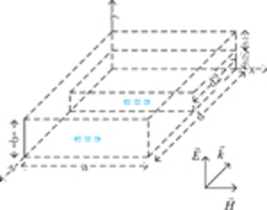
Figure 1: Apertured enclosure with an interior enclosure on bottom tail-end and the coordinate system, all apertures are positioned centrally in the walls.

The geometry of the apertured enclosure with an interior enclosure on the bottom tail-end illuminated by an external plane wave is shown in Fig. 1. The overall size of the enclosure is $a\times b\times d$ mm, and the size of the interior enclosure is $a\times b_2\times d_2$ mm.

The size of the aperture on the front wall and interior wall are $l\times w$ and $l_2\times w_2$ respectively, and its central point locates at the center of the wall. Additionally, the monitor point P inside the enclosure has the coordinates of $(x_p,y_p,z_p)$. In this paper, we divided the inner structure of the mentioned enclosure in Fig. 1 into three part: the space 1 in front of the interior enclosure, the interior enclosure 2, and the space 3 adjacent to the interior enclosure 2.

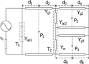
Figure 2: Equivalent circuit of the enclosure.

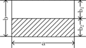
Figure 3: Cross sectional view of the obstacle, the shadow part is the front wall of the interior enclosure.

The equivalent circuit of the enclosure in Fig. 1 is given in Fig. 2. The side wall is treated as waveguide, then the impedance and propagation constant $z_g$ and $k_g$ are given by:

$$Z_g=Z_0/\sqrt{1-{(\frac{m\lambda }{2a})}^2-{(\frac{n\lambda }{2b})}^2},$$

(1)

$$k_g=k_0\sqrt{1-{(\frac{m\lambda }{2a})}^2-{(\frac{n\lambda }{2b})}^2}.$$

(2)

The radiating source is represented by voltage $V_0$ and impedance of free space $Z_0=377\mathrm{\Omega }$. The apertures are treated as a coplanar strip transmission line which shorted at each end, its characteristic impedance is given by Gupta et al [18]:

$$Z_{ap}=\frac{j}{2}\frac{l}{a}{Z}_{os}tan(\frac{k_{0}l}{2}).$$

(3)

$Z_{os}$ is the aperture characteristic impedance:

$$Z_{os}=120{\pi }^2[\ln (2\frac{1+\sqrt[4]{1-{(w_e/b)}^2}}{1-\sqrt[4]{1-{(w_e/b)}^2}})].$$

(4)

Since the enclosure have a thickness, when the $w_e⩽\frac{b}{\sqrt{2}}$, we have effective width $w_e$ :

$$w_e=w-\frac{5t}{4\pi }[1+\ln \frac{4\pi w}{t}],$$

(5)

where t represents enclosure wall’s thickness, w is the width of the slot.

The aperture on the inner enclosure also calculated by Equation 3, where b is replaced by $b_2$.

In this paper, we modeled the front wall of the interior enclosure as a junction between two different rectangular waveguides, as shown in Fig. 2, when the height of rear waveguide is nearly half of the front one, the equivalent impedance can be writen as [19]:

$Y_w={\displaystyle \frac{4j{b}_1}{Z_g{\lambda }_g}}[ln({\displaystyle \frac{1-{\alpha }^2}{4\alpha }}){({\displaystyle \frac{1+\alpha }{1-\alpha }})}^{\frac{1}{2}(\alpha +(1/\alpha ))}+{\displaystyle \frac{2}{A}}],$	(6)
$A={({\displaystyle \frac{1+\alpha }{1-\alpha }})}^{2\alpha }{\displaystyle \frac{1+\sqrt{1-{(2b_1/{\lambda }_g)}^2}}{1-\sqrt{1-{(2b_1/{\lambda }_g)}^2}}}-{\displaystyle \frac{1+3{\alpha }^2}{1-{\alpha }^2}},$

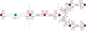
Figure 4: Signal flow graph of the enclosure.

where $\alpha =b_2/b$. Figure 4 gives electromagnetic topology for the enclosure shown in Fig. 1. Node $N_1$ represents the monitor point in free space, and nodes $N_3$, $N_5$, $N_7$ denote monitor points $P_1$, $P_2$ and $P_3$ inside the sub-enclosures respectively. The aperture on the front wall is represented by nodes $N_2$, he aperture on the interior wall and the window are represented by node $N_4$ as a three ports network, and the shorted end of enclosure 2 and space 3 is represented by $N_6,N_8$. The monitor point $N_1$ in free space and shorted ends $N_6,N_8$ are equivalented by a one-port network. Tube 1 denotes the electromagnetic wave propagation in free space, while Tube 2, Tube 3, Tube 4, and Tube 6 are the wave propagation between the monitor points and the apertures/window in sub-enclosures. Tube 5 and Tube 7 denote the wave propagation to the short end of enclosure 2 and space 3 respectively.

The extended BLT equation can be expressed as [10]:

$$\mathbf{V}=(\mathbf{E}+\mathbf{S})\times {(\mathbf{\Gamma }-\mathbf{S})}^{-\mathbf{1}}\times {\mathbf{V}}_{\mathbf{s}},$$

(7)

where $\mathbf{V}$ is the voltage response matrix, $\mathbf{E}$ is the unit matrix, $\mathbf{S}$ is the scattering parameter matrix, $\mathbf{\Gamma }$ represents the propagation matrix, and ${\mathbf{V}}_{\mathbf{s}}$ represents the source matrix.

Based on Fig. 4, the propagation equation can be given by:

$$\left[\begin{array}{c}\hfill V_{1,1}^{ref}\hfill \\ \hfill V_{1,2}^{ref}\hfill \\ \hfill V_{2,2}^{ref}\hfill \\ \hfill V_{2,3}^{ref}\hfill \\ \hfill V_{3,3}^{ref}\hfill \\ \hfill V_{3,4}^{ref}\hfill \\ \hfill V_{4,4}^{ref}\hfill \\ \hfill V_{6,4}^{ref}\hfill \\ \hfill V_{4,5}^{ref}\hfill \\ \hfill V_{5,5}^{ref}\hfill \\ \hfill V_{5,6}^{ref}\hfill \\ \hfill V_{6,7}^{ref}\hfill \\ \hfill V_{7,7}^{ref}\hfill \\ \hfill V_{7,8}^{ref}\hfill \end{array}\right]=\left[\begin{array}{cccccccccccccc}\hfill 0\hfill & \hfill e^{{\gamma }_0{l}_x}\hfill & \hfill 0\hfill & \hfill 0\hfill & \hfill 0\hfill & \hfill 0\hfill & \hfill 0\hfill & \hfill 0\hfill & \hfill 0\hfill & \hfill 0\hfill & \hfill 0\hfill & \hfill 0\hfill & \hfill 0\hfill & \hfill 0\hfill \\ \hfill e^{{\gamma }_0{l}_x}\hfill & \hfill 0\hfill & \hfill 0\hfill & \hfill 0\hfill & \hfill 0\hfill & \hfill 0\hfill & \hfill 0\hfill & \hfill 0\hfill & \hfill 0\hfill & \hfill 0\hfill & \hfill 0\hfill & \hfill 0\hfill & \hfill 0\hfill & \hfill 0\hfill \\ \hfill 0\hfill & \hfill 0\hfill & \hfill 0\hfill & \hfill e^{g_1{d}_1}\hfill & \hfill 0\hfill & \hfill 0\hfill & \hfill 0\hfill & \hfill 0\hfill & \hfill 0\hfill & \hfill 0\hfill & \hfill 0\hfill & \hfill 0\hfill & \hfill 0\hfill & \hfill 0\hfill \\ \hfill 0\hfill & \hfill 0\hfill & \hfill e^{g_1{d}_1}\hfill & \hfill 0\hfill & \hfill 0\hfill & \hfill 0\hfill & \hfill 0\hfill & \hfill 0\hfill & \hfill 0\hfill & \hfill 0\hfill & \hfill 0\hfill & \hfill 0\hfill & \hfill 0\hfill & \hfill 0\hfill \\ \hfill 0\hfill & \hfill 0\hfill & \hfill 0\hfill & \hfill 0\hfill & \hfill 0\hfill & \hfill e^{g_1{d}_2}\hfill & \hfill 0\hfill & \hfill 0\hfill & \hfill 0\hfill & \hfill 0\hfill & \hfill 0\hfill & \hfill 0\hfill & \hfill 0\hfill & \hfill 0\hfill \\ \hfill 0\hfill & \hfill 0\hfill & \hfill 0\hfill & \hfill 0\hfill & \hfill e^{g_1{d}_2}\hfill & \hfill 0\hfill & \hfill 0\hfill & \hfill 0\hfill & \hfill 0\hfill & \hfill 0\hfill & \hfill 0\hfill & \hfill 0\hfill & \hfill 0\hfill & \hfill 0\hfill \\ \hfill 0\hfill & \hfill 0\hfill & \hfill 0\hfill & \hfill 0\hfill & \hfill 0\hfill & \hfill 0\hfill & \hfill 0\hfill & \hfill 0\hfill & \hfill e^{g_2{d}_3}\hfill & \hfill 0\hfill & \hfill 0\hfill & \hfill 0\hfill & \hfill 0\hfill & \hfill 0\hfill \\ \hfill 0\hfill & \hfill 0\hfill & \hfill 0\hfill & \hfill 0\hfill & \hfill 0\hfill & \hfill 0\hfill & \hfill 0\hfill & \hfill 0\hfill & \hfill 0\hfill & \hfill 0\hfill & \hfill 0\hfill & \hfill e^{g_2{d}_4}\hfill & \hfill 0\hfill & \hfill 0\hfill \\ \hfill 0\hfill & \hfill 0\hfill & \hfill 0\hfill & \hfill 0\hfill & \hfill 0\hfill & \hfill 0\hfill & \hfill e^{g_2{d}_3}\hfill & \hfill 0\hfill & \hfill 0\hfill & \hfill 0\hfill & \hfill 0\hfill & \hfill 0\hfill & \hfill 0\hfill & \hfill 0\hfill \\ \hfill 0\hfill & \hfill 0\hfill & \hfill 0\hfill & \hfill 0\hfill & \hfill 0\hfill & \hfill 0\hfill & \hfill 0\hfill & \hfill 0\hfill & \hfill 0\hfill & \hfill 0\hfill & \hfill e^{g_3{d}_5}\hfill & \hfill 0\hfill & \hfill 0\hfill & \hfill 0\hfill \\ \hfill 0\hfill & \hfill 0\hfill & \hfill 0\hfill & \hfill 0\hfill & \hfill 0\hfill & \hfill 0\hfill & \hfill 0\hfill & \hfill 0\hfill & \hfill 0\hfill & \hfill e^{g_3{d}_5}\hfill & \hfill 0\hfill & \hfill 0\hfill & \hfill 0\hfill & \hfill 0\hfill \\ \hfill 0\hfill & \hfill 0\hfill & \hfill 0\hfill & \hfill 0\hfill & \hfill 0\hfill & \hfill 0\hfill & \hfill 0\hfill & \hfill e^{g_2{d}_4}\hfill & \hfill 0\hfill & \hfill 0\hfill & \hfill 0\hfill & \hfill 0\hfill & \hfill 0\hfill & \hfill 0\hfill \\ \hfill 0\hfill & \hfill 0\hfill & \hfill 0\hfill & \hfill 0\hfill & \hfill 0\hfill & \hfill 0\hfill & \hfill 0\hfill & \hfill 0\hfill & \hfill 0\hfill & \hfill 0\hfill & \hfill 0\hfill & \hfill 0\hfill & \hfill 0\hfill & \hfill e^{g_3{d}_6}\hfill \\ \hfill 0\hfill & \hfill 0\hfill & \hfill 0\hfill & \hfill 0\hfill & \hfill 0\hfill & \hfill 0\hfill & \hfill 0\hfill & \hfill 0\hfill & \hfill 0\hfill & \hfill 0\hfill & \hfill 0\hfill & \hfill 0\hfill & \hfill e^{g_3{d}_6}\hfill & \hfill 0\hfill \end{array}\right]\left[\begin{array}{c}\hfill V_{1,1}^{inc}\hfill \\ \hfill V_{1,2}^{inc}\hfill \\ \hfill V_{2,2}^{inc}\hfill \\ \hfill V_{2,3}^{inc}\hfill \\ \hfill V_{3,3}^{inc}\hfill \\ \hfill V_{3,4}^{inc}\hfill \\ \hfill V_{4,4}^{inc}\hfill \\ \hfill V_{6,4}^{inc}\hfill \\ \hfill V_{4,5}^{inc}\hfill \\ \hfill V_{5,5}^{inc}\hfill \\ \hfill V_{5,6}^{inc}\hfill \\ \hfill V_{6,7}^{inc}\hfill \\ \hfill V_{7,\mathrm{`}7}^{inc}\hfill \\ \hfill V_{7,8}^{inc}\hfill \end{array}\right]-\left[\begin{array}{c}\hfill V_0\hfill \\ \hfill 0\hfill \\ \hfill 0\hfill \\ \hfill 0\hfill \\ \hfill 0\hfill \\ \hfill 0\hfill \\ \hfill 0\hfill \\ \hfill 0\hfill \\ \hfill 0\hfill \\ \hfill 0\hfill \\ \hfill 0\hfill \\ \hfill 0\hfill \\ \hfill 0\hfill \\ \hfill 0\hfill \end{array}\right]$$

(8)

$l_x$ is the distance between electromagnetic wave and the aperture on the front wall; ${\gamma }_0=j{k}_0$ is the phase constant of freespace. Where $g_i=j{k}_0\sqrt{1-{(m\lambda /2a_i)}^2-{(n\lambda /2b_i)}^2}$, i is the number of the space/enclosure, $d_j$ shown in Fig. 2 represent the distance between each point in the planar wave propagation direction.

The scattering equation contains the scattering matrix $\mathbf{S}$ is given by:

$$\left[\begin{array}{c}\hfill V_{1,1}^{ref}\hfill \\ \hfill V_{1,2}^{ref}\hfill \\ \hfill V_{2,2}^{ref}\hfill \\ \hfill V_{2,3}^{ref}\hfill \\ \hfill V_{3,3}^{ref}\hfill \\ \hfill V_{3,4}^{ref}\hfill \\ \hfill V_{4,4}^{ref}\hfill \\ \hfill V_{6,4}^{ref}\hfill \\ \hfill V_{4,5}^{ref}\hfill \\ \hfill V_{5,5}^{ref}\hfill \\ \hfill V_{5,6}^{ref}\hfill \\ \hfill V_{6,7}^{ref}\hfill \\ \hfill V_{7,7}^{ref}\hfill \\ \hfill V_{7,8}^{ref}\hfill \end{array}\right]=\left[\begin{array}{cccccccccccccc}\hfill {\rho }^1\hfill & \hfill 0\hfill & \hfill 0\hfill & \hfill 0\hfill & \hfill 0\hfill & \hfill 0\hfill & \hfill 0\hfill & \hfill 0\hfill & \hfill 0\hfill & \hfill 0\hfill & \hfill 0\hfill & \hfill 0\hfill & \hfill 0\hfill & \hfill 0\hfill \\ \hfill 0\hfill & \hfill S_{11}^2\hfill & \hfill S_{12}^2\hfill & \hfill 0\hfill & \hfill 0\hfill & \hfill 0\hfill & \hfill 0\hfill & \hfill 0\hfill & \hfill 0\hfill & \hfill 0\hfill & \hfill 0\hfill & \hfill 0\hfill & \hfill 0\hfill & \hfill 0\hfill \\ \hfill 0\hfill & \hfill S_{21}^2\hfill & \hfill S_{22}^2\hfill & \hfill 0\hfill & \hfill 0\hfill & \hfill 0\hfill & \hfill 0\hfill & \hfill 0\hfill & \hfill 0\hfill & \hfill 0\hfill & \hfill 0\hfill & \hfill 0\hfill & \hfill 0\hfill & \hfill 0\hfill \\ \hfill 0\hfill & \hfill 0\hfill & \hfill 0\hfill & \hfill S_{11}^3\hfill & \hfill S_{12}^3\hfill & \hfill 0\hfill & \hfill 0\hfill & \hfill 0\hfill & \hfill 0\hfill & \hfill 0\hfill & \hfill 0\hfill & \hfill 0\hfill & \hfill 0\hfill & \hfill 0\hfill \\ \hfill 0\hfill & \hfill 0\hfill & \hfill 0\hfill & \hfill S_{21}^3\hfill & \hfill S_{22}^3\hfill & \hfill 0\hfill & \hfill 0\hfill & \hfill 0\hfill & \hfill 0\hfill & \hfill 0\hfill & \hfill 0\hfill & \hfill 0\hfill & \hfill 0\hfill & \hfill 0\hfill \\ \hfill 0\hfill & \hfill 0\hfill & \hfill 0\hfill & \hfill 0\hfill & \hfill 0\hfill & \hfill S_{11}^4\hfill & \hfill S_{12}^4\hfill & \hfill S_{13}^4\hfill & \hfill 0\hfill & \hfill 0\hfill & \hfill 0\hfill & \hfill 0\hfill & \hfill 0\hfill & \hfill 0\hfill \\ \hfill 0\hfill & \hfill 0\hfill & \hfill 0\hfill & \hfill 0\hfill & \hfill 0\hfill & \hfill S_{21}^4\hfill & \hfill S_{22}^4\hfill & \hfill S_{23}^4\hfill & \hfill 0\hfill & \hfill 0\hfill & \hfill 0\hfill & \hfill 0\hfill & \hfill 0\hfill & \hfill 0\hfill \\ \hfill 0\hfill & \hfill 0\hfill & \hfill 0\hfill & \hfill 0\hfill & \hfill 0\hfill & \hfill S_{31}^4\hfill & \hfill S_{32}^4\hfill & \hfill S_{33}^4\hfill & \hfill 0\hfill & \hfill 0\hfill & \hfill 0\hfill & \hfill 0\hfill & \hfill 0\hfill & \hfill 0\hfill \\ \hfill 0\hfill & \hfill 0\hfill & \hfill 0\hfill & \hfill 0\hfill & \hfill 0\hfill & \hfill 0\hfill & \hfill 0\hfill & \hfill 0\hfill & \hfill S_{11}^5\hfill & \hfill S_{12}^5\hfill & \hfill 0\hfill & \hfill 0\hfill & \hfill 0\hfill & \hfill 0\hfill \\ \hfill 0\hfill & \hfill 0\hfill & \hfill 0\hfill & \hfill 0\hfill & \hfill 0\hfill & \hfill 0\hfill & \hfill 0\hfill & \hfill 0\hfill & \hfill S_{21}^5\hfill & \hfill S_{22}^5\hfill & \hfill 0\hfill & \hfill 0\hfill & \hfill 0\hfill & \hfill 0\hfill \\ \hfill 0\hfill & \hfill 0\hfill & \hfill 0\hfill & \hfill 0\hfill & \hfill 0\hfill & \hfill 0\hfill & \hfill 0\hfill & \hfill 0\hfill & \hfill 0\hfill & \hfill 0\hfill & \hfill {\rho }^6\hfill & \hfill 0\hfill & \hfill 0\hfill & \hfill 0\hfill \\ \hfill 0\hfill & \hfill 0\hfill & \hfill 0\hfill & \hfill 0\hfill & \hfill 0\hfill & \hfill 0\hfill & \hfill 0\hfill & \hfill 0\hfill & \hfill 0\hfill & \hfill 0\hfill & \hfill 0\hfill & \hfill S_{11}^7\hfill & \hfill S_{12}^7\hfill & \hfill 0\hfill \\ \hfill 0\hfill & \hfill 0\hfill & \hfill 0\hfill & \hfill 0\hfill & \hfill 0\hfill & \hfill 0\hfill & \hfill 0\hfill & \hfill 0\hfill & \hfill 0\hfill & \hfill 0\hfill & \hfill 0\hfill & \hfill S_{21}^7\hfill & \hfill S_{22}^7\hfill & \hfill 0\hfill \\ \hfill 0\hfill & \hfill 0\hfill & \hfill 0\hfill & \hfill 0\hfill & \hfill 0\hfill & \hfill 0\hfill & \hfill 0\hfill & \hfill 0\hfill & \hfill 0\hfill & \hfill 0\hfill & \hfill 0\hfill & \hfill 0\hfill & \hfill 0\hfill & \hfill {\rho }^8\hfill \end{array}\right]\left[\begin{array}{c}\hfill V_{1,1}^{inc}\hfill \\ \hfill V_{1,2}^{inc}\hfill \\ \hfill V_{2,2}^{inc}\hfill \\ \hfill V_{2,3}^{inc}\hfill \\ \hfill V_{3,3}^{inc}\hfill \\ \hfill V_{3,4}^{inc}\hfill \\ \hfill V_{4,4}^{inc}\hfill \\ \hfill V_{6,4}^{inc}\hfill \\ \hfill V_{4,5}^{inc}\hfill \\ \hfill V_{5,5}^{inc}\hfill \\ \hfill V_{5,6}^{inc}\hfill \\ \hfill V_{6,7}^{inc}\hfill \\ \hfill V_{7,\mathrm{`}7}^{inc}{V}_{7,8}^{inc}\hfill \end{array}\right]$$

(9)

${\rho }^1=0$ is the free space, and ${\rho }^6={\rho }^8=-1$ are the short ends. $S^3$ , $S^4$ and $S^5$ represents $p_1$ , $p_2$ and $p_3$:

$$S^3=S^5=S^7=\left[\begin{array}{cc}\hfill 0\hfill & \hfill 1\hfill \\ \hfill 1\hfill & \hfill 0\hfill \end{array}\right].$$

(10)

$S^2$ can be obtained from network $T_1$ in Fig 2:

$$S^2=\left[\begin{array}{cc}\hfill \frac{Y_0-Y_{g1}-Y_{ap1}}{Y_0+Y_{g1}+Y_{ap1}}\hfill & \hfill \frac{2Y_{g1}}{Y_0+Y_{g1}+Y_{ap1}}\hfill \\ \hfill \frac{2Y_0}{Y_0+Y_{g1}+Y_{ap1}}\hfill & \hfill \frac{Y_{g1}-Y_0-Y_{ap1}}{Y_0+Y_{g1}+Y_{ap1}}\hfill \end{array}\right].$$

(11)

We neglect the coupling between aperture 2 and window 1, assume that $S_{23}^4=S_{32}^4=0$ then $S^4$ is:

$S_{11}^4=(Y_{g1}{Y}_{g3}+Y_{g1}{Y}_w+Y_{g1}{Y}_{ap2}+Y_{g1}{Y}_{g2}$

$-Y_{g3}{Y}_{g2}-Y_w{Y}_{g2}-Y_{ap2}{Y}_{g3}-Y_{ap2}{Y}_w)/Y{}_t{}^4,$

$S_{12}^4=2(Y_{g1}{Y}_{g3}+Y_{g1}{Y}_w)/Y_t^4,$

$S_{13}^4=2(Y_{g1}{Y}_{g2}+Y_{g1}{Y}_{ap2})/Y_t^4,$

$S_{21}^4=2(Y_{g1}{Y}_{g2}+Y_{g2}{Y}_{g3}+Y_{g2}{Y}_w)/Y_t^4,$

$S_{22}^4=(Y_{g1}{Y}_{g2}+Y_{g2}{Y}_{g3}+Y_{g2}{Y}_w-Y_{g1}{Y}_{ap2}$

$-Y_{g3}{Y}_{ap2}-Y_{ap2}{Y}_w-Y_{g1}{Y}_w-Y_{g1}{Y}_{g3})/Y{}_t{}^4,$

$S_{31}^4=2(Y_{g1}{Y}_{g3}+Y_{g2}{Y}_{g3}+Y_{g3}{Y}_{ap2})/Y_t^4,$

$S_{33}^4=(Y_{g1}{Y}_{g3}+Y_{g2}{Y}_{g3}+Y_{g3}{Y}_{ap2}-Y_{g1}{Y}_w-$

$Y_{g2}{Y}_w-Y_{g1}{Y}_w-Y_{g1}{Y}_{g2}-Y_{ap2}{Y}_w)/Y{}_t{}^4,$

$Y_t^4=Y_{g1}{Y}_{g3}+Y_{g1}{Y}_w+Y_{g1}{Y}_{ap2}+Y_{g1}{Y}_{g2}$

$+Y_{g2}{Y}_{g3}+Y_{g2}{Y}_w+Y_{g3}{Y}_{ap2}+Y_{ap2}{Y}_w,$

where $Y_0$, $Y_g$, $Y_{ap}$, and $Y_w$ are the admittances of free space, rectangular waveguide, aperture and window respectively, and $Y_0=\frac{1}{Z_0},Y_g=\frac{1}{Z_g},Yap=\frac{1}{Z_{ap}},Y_w=\frac{1}{Z_w}.$

Then the SE at point P is calculated by $SE=-20log(V_p/V_0)$.

III. RESULTS AND DISCUSSION

In this section, the enclosure with an interior enclosure on bottom tail-end are performed to validate the proposed model, the simulation results of the proposed model are compared with the CST-MS software. The walls of the enclosure are assumed to be perfectly conducting, and their thicknesses are defined as 1 mm.

A. Verification for the apertured enclosure with an interior enclosure on bottom tail-end

It is assumed that the dimensions of enclosure shown in Fig. 1 are 200 mm × 120 mm × 600 mm, $b_1=b_2=60mm$, other parameter settings of case 1 are listed in Table 1, including the enclosure dimensions, the aperture size, and the monitor point positions.

Table 1: Parametars of the enclosure

No	Enclosure	Aperture	Monitor point
1	200 × 120 × 300	60 × 10	100, 60, 450
2	200 × 60 × 300	50 × 10	100, 30, 150
3	200 × 60 × 300		100, 90, 150

Figures 5 to 7 show the SE results of monitor point $P_1$, $P_2$, and $P_3$ obtained by the CST and the proposed method, respectively. The discontinuity in the curve is due to removing the frequency point having a term with a zero denominator in the calculation process. It is observed that the SE results given by these two methods are match up relatively well, indicating that the proposed model is effective in predicting the SE and resonances of a metallic enclosure with an interior enclosure. Besides, in a wide frequency range near the resonant frequency of the enclosure, the SE changes dramatically, and even appears negative values. The physical significance of these values indicates that the apertured enclosure has the worst shielding performance in this condition, and the above phenomenon should be attributed to the resonance effect.

Figure 5: Comparison between the SE result from proposed method with result of CST for observe point 1.

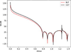
Figure 6: Comparison between the SE result from proposed method with result of CST for observe point 2.

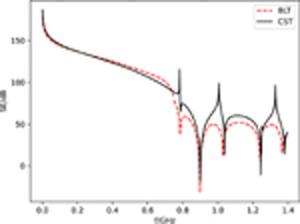
Figure 7: Comparison between the SE result from proposed method with result of CST for observe point 3.

From the comparison between the SE results from different enclosures, it can be seen that: (1) as a double shield enclosure, enclosure 2 has the best shielding performance; (2) a more pronounced deviation can be seen in enclosure 2, the potential reason may be due to the reflection and diffraction between aperture and the window structure. Such reflection are likely to have influenced the results in enclosure 1. Also, the aperture scattering matrix of junction $N_4$ cannot fully consider the direct electromagnetic coupling between the the aperture of enclosure 2 and the window of space 3.

B. Parameter analysis

Since the method proposed in this paper can efficiently calculate the shielding effectiveness, in the following discussion, the proposed method is employed to analyze the effect of dimensional variation on shielding effectivenes.

Figure 8 demonstrates the effect of enclosure width $a$ on the shielding effectiveness in space 1. Except for the enclosure width, all parameters are the same as the case mentioned before, and the enclosure widths represented by the three sets of curves in the Fig. 8 are 300, 320, and 340 mm, respectively, while the observation point is always located in the middle of the enclosure. It can be seen that the enclosure width changes have a great influence on the resonant point frequency and shielding effectiveness, which will cause the frequency shift of the resonant point. As the cavity width increases, the resonant point frequency will be reduced.

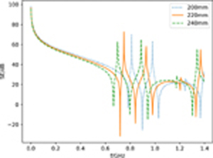
Figure 8: Effect of enclosure width variation on shielding effectiveness in space 1.

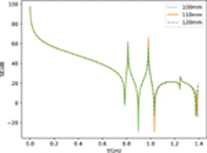
Figure 9: Effect of enclosure height variation on shielding effectiveness in space 1.

Figure 9 demonstrates the effect of enclosure height $b$ variation on shielding effectiveness in space 1. Due to the direction of the electric field of the incident wave, the effect of height variation on shielding performance and resonant frequency is very small.

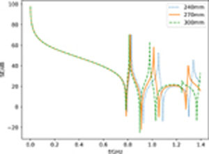
Figure 10: Effect of rear enclosure depth variation on shielding effectiveness in space 1.

Figure 10 demonstrates the effect of the variation of the rear depth $d_2$ on the shielding effectiveness in space 1. All parameters are the same as the case mentioned before except for the rear depth, and the depths $d_2$ represented by the three sets of curves in the Fig. 10 are 240, 270, and 300 mm, respectively, while the observation point is always located in the middle of space 1. It can be seen that as the depth of the rear enclosure increases, the shielding effectiveness increases at lower frequencies, and the resonant frequency also shifts to lower frequencies as the depth of the rear enclosure increases, which leads to a decrease in shielding effectiveness in some frequency bands above the cutoff frequency.

All the cases are computed on the same computer, which has a 2.2-GHz Intel i7-8750 CPU. The CST takes 20 minutes to complete a 200 frequency point simulation, while the fast algorithm takes no more than 0.2 s for the same case, indicating the high computational efficiency of the fast algorithm compared with the CST simulation.

IV. CONCLUSION

A method based on the EMT theory and BLT equation is presented to analyze the shielding performance of an apertured enclosure with an interior enclosure illuminated by an external plane wave. By modeling the front wall of the interior enclosure as a junction between two different rectangular waveguides, we derive a three-port scattering matrix from describing the coupling relation between the interior enclosure and the adjacent space. The total electric field can be derived from the relation between voltage response and field distribution inside the enclosure. This method proves that the BLT equation can handle complex enclosures by modifying the electromagnetic topology relationship. Several monitor points are presented to demonstrate the validity and accuracy of this method. The results indicate that the proposed method has a good agreement with numerical methods over a wide frequency range while it can dramatically improve the calculation speed. The proposed algorithm can be used to perform fast calculations on the effect of enclosure dimensions on shielding effectiveness. We investigated the effect of dimensional parameters on the shielding effectiveness of the enclosure. We found that due to the electric field direction, the variation of enclosure height can hardly affects the shielding effectiveness.

REFERENCES

[1] J. Bridges, “Proposed recommended practices for the measurement of shielding effectiveness of high-performance shielding enclosures,” IEEE Trans. Electromagn. Compat, vol. EMC-10, no. 1, pp. 82-94, 1968.

[2] S. Georgakopoulos, C. Birtcher, and C. Balanis, “HIRF penetration through apertures: FDTD versus measurements,” IEEE Trans. Electromagn. Compat, vol. 43, no. 3, pp. 282-294, 2001.

[3] R. Araneo and G. Lovat, “Fast MoM analysis of the shielding effectiveness of rectangular enclosures with apertures, metal plates, and conducting objects,” IEEE Trans. Electromagn. Compat, vol. 51, no. 2, pp. 274-283, 2009.

[4] B. Audone and M. Balma, “Shielding effectiveness of apertures in rectangular cavities,” IEEE Trans. Electromagn. Compat, vol. 31, no. 1, pp. 102-106, 1989.

[5] B.-L. Nie, P.-A. Du, Y.-T. Yu, and Z. Shi, “Study of the shielding properties of enclosures with apertures at higher frequencies using the transmission-line modeling method,” IEEE Trans. Electromagn. Compat, vol. 53, no. 1, pp. 73-81, 2011.

[6] Z. Kubík and J. Skála, “Shielding effectiveness simulation of small perforated shielding enclosures using FEM,” Energies, vol. 9, no. 3, p. 129, 2016.

[7] M. P. Robinson, T. M. Benson, C. Christopoulos, J. F. Dawson, M. D. Ganley, A. C. Marvin, S. J. Porter, and D. W. P. Thomas, “Analytical formulation for the shielding effectiveness of enclosures with apertures,” IEEE Trans. Electromagn. Compat, vol. 40, no. 3, p. 9, 1998.

[8] M. P. Robinson, J. D. Turner, D. W. P. Thomas, J. F. Dawson, M. D. Ganley, A. C. Marvin, S. J. Porter, T. M. Benson, and C. Christopoulos, “Shielding effectiveness of a rectangular enclosure with a rectangular aperture,” Electronics Letters, vol. 32, no. 17, pp. 1559-1560, 1996.

[9] F. Tesche, “Topological concepts for internal EMP interaction,” IEEE Trans. Antennas. Propagat, vol. 26, no. 1, pp. 60-64, 1978.

[10] F. M. Tesche, J. M. Keen, and C. M. Butler, “Example of the use of the BLT equation for EM field propagation and coupling calculations,” URSI Radio Science Bulletin, vol. 2005, no. 312, pp. 32-47, 2005.

[11] F. M. Tesche, “On the analysis of a transmission line with nonlinear trerminations using the time-dependent BLT equation,” IEEE Trans. Electromagn. Compat, vol. 49, no. 2, pp. 427-433, 2007.

[12] B.-L. Nie and P.-A. Du, “An efficient and reliable circuit model for the shielding effectiveness prediction of an enclosure with an aperture,” IEEE Trans. Electromagn. Compat, vol. 57, no. 3, pp. 357-364, 2015.

[13] M.-C. Yin and P.-A. Du, “An improved circuit model for the prediction of the shielding effectiveness and resonances of an enclosure with apertures,” IEEE Trans. Electromagn. Compat, vol. 58, no. 2, pp. 448-456, 2016.

[14] P. Dehkhoda, A. Tavakoli, and R. Moini, “An efficient and reliable shielding effectiveness evaluation of a rectangular enclosure with numerous apertures,” IEEE Trans. Electromagn. Compat, vol. 50, no. 1, pp. 208-212, 2008.

[15] Y. Gong and B. Wang, “An efficient method for predicting the shielding effectiveness of an enclosure with multiple apertures,” J. Electromagn. Waves Appl, vol. 34, no. 8, pp. 1057-1072, 2020.

[16] J. Sun, Y. Gong, and L. Jiang, “An improved model for the analysis of the shielding performance of an apertured enclosure based on EMT theory and BLT equation,” J. Electromagn. Waves Appl, vol. 36, no. 2, pp. 246-260, 2022.

[17] Y. Kan, L.-P. Yan, X. Zhao, H.-J. Zhou, Q. Liu, and K.-M. Huang, “Electromagnetic topology based fast algorithm for shielding effectiveness estimation of multiple enclosures with apertures,” Acta Phys Sin, vol. 65, no. 3, p. 030702, 2016.

[18] K. Gupta, R. Garg, I. Bahl, and P. Bhartia, Coplanar Lines: Coplanar Waveguide and Coplanar Strips, vol. 2, Artech House, 1996.

[19] N. Marcuvitz, Waveguide Handbook, Institution of Electrical Engineers, 1986.

BIOGRAPHIES

Jin-Cheng Zhou was born in Jiangsu, China, in 1990. He received a B.A. degree in Xi’an Technological University, China in 2008. He is currently working on his Ph.D. at the School of Information and Electronics of Beijing Institute of Technology. His research interests include radio propagation, EMC, and EM protection.

Xue-Tian Wang was born in Jiangsu, China, in 1961. He received a Ph.D. from the Department of Electronic Engineering of Beijing Institute of Technology in 2002. He has been working at Beijing Institute of Technology as a researcher since August 2001, and he has been a professor since 2003. His research interests include EMC, EM protection, and electromagnetic radiation characteristics.

ACES JOURNAL, Vol. 37, No. 10, 1014–1020
doi: 10.13052/2022.ACES.J.371001
© 2022 River Publishers

ABSTRACT

I. INTRODUCTION

II. ELECTROMAGNETIC TOPOLOGICAL MODEL

III. RESULTS AND DISCUSSION

A. Verification for the apertured enclosure with an interior enclosure on bottom tail-end

B. Parameter analysis

IV. CONCLUSION

REFERENCES

BIOGRAPHIES