Antenna Synthesis by Levin’s Method using a Novel Optimization Algorithm for Knot Placement

Goker Sener

Department of Electrical-Electronics Engineering
Cankaya University, Ankara, 06790, Turkey
sener@cankaya.edu.tr

Submitted On: September 25, 2022; Accepted On: February 20, 2023

ABSTRACT

Antenna synthesis refers to determining the antenna current distribution by evaluating the inverse Fourier integral of its radiation pattern. Since this integral is highly oscillatory, Levin’s method can be used for the solution, providing high accuracy. In Levin’s method, the integration domain is divided into equally spaced sub-intervals, and the integrals are solved by transferring them into differential equations. This article uses a new optimization algorithm to determine the location of these interval points (knots) to improve the method’s accuracy. Two different antenna design examples are presented to validate the accuracy and efficiency of the proposed method for antenna synthesis applications.

Index Terms: antenna synthesis, fourier integral, highly oscillatory integrals knot placement, Levin’s method.

I. INTRODUCTION

Antenna synthesis aims to find the current distribution by evaluating the inverse Fourier integral of the antenna radiation pattern. [1, 2]. Since this integral is highly oscillatory, a proper solution algorithm must be employed [3, 4].

Levin’s method is a numerical technique widely used for solving highly oscillatory integrals, and it gives accurate results, especially with complex phase functions [4, 5, 6, 7]. In this method, the integral domain is divided into equally spaced sub-intervals, and the integrals of these sub-intervals are evaluated by transferring them into differential equations. These equations are then solved by converting the problem into a linear equation system by the collocation method. Lastly, the results of the sub-integrals are added to obtain the final solution.

The collocation approximation is the finite sum of some linearly independent basis functions with unknown coefficients. Therefore, selecting the basis functions is highly important regarding the method’s accuracy. In [8], Levin’s method is used with “reproducing kernel functions”, giving better accuracy and stability than the other well-known basis functions.

In this paper, the Levin’s method is improved by using a new optimization algorithm to determine the locations of the integration sub-interval points (knots). This algorithm was first introduced by Yeh et al. in [9] as a knot placement method for the B-spline curve fitting. Here, it is used in the Levin’s method to obtain higher accuracy. To the author’s knowledge, this is the first time the Levin’s method is used with this new knot optimization technique in an antenna synthesis application.

Two examples are presented to validate the accuracy and efficiency of the proposed method. In the first example, the radiation pattern of a log-periodic antenna, 4030/LP/10, is used to obtain the equivalent current distribution on a linear conductor. In the second example, an array antenna with a narrow beamwidth is considered. The error and stability analyses are carried out by comparing the original radiation patterns with the ones obtained by the proposed solution. The results show that the proposed method provides more accuracy than the standard equal-distance knot placement integration technique, particularly for narrow beam radiation.

The remaining of this paper is arranged as follows: In sections II and III, the Levin’s method and reproducing kernel functions are explained, respectively. In section IV, the novel knot placement method is explained. In section V, the antenna synthesis examples are presented. In section VI, conclusions are made based on the error and stability analysis results.

II. LEVIN’S METHOD

Levin’s method is a numerical technique to solve highly oscillatory integrals in the form:

$$I={\int }_a^{b}f(x)e^{iq(x)}\mathit{d}x,$$

(1)

where $f(x)$ is a slowly varying function, and $q(x)$ is a highly oscillatory function. Since $q(x)$ is oscillatory, it can be written that $|q^{\prime }(x)|\gg {(b-a)}^{-1}$.

In Levin’s method, the integral in (1) is transformed into the following differential equation:

$$f(x)=i{q}^{\prime }(x)p(x)+p^{\prime }(x)=L^{(1)}p(x).$$

(2)

Substituting (2) in (1) yields:

$$\begin{array}{cc}\hfill I& ={\int }_a^b\left(i{q}^{\prime }(x)p(x)+p^{\prime }(x)\right)e^{iq(x)}\mathit{d}x\hfill \\ & ={\int }_a^b\frac{d}{dx}\left(p(x)e^{iq(x)}\right)\mathit{d}x\hfill \\ & =p(b)e^{iq(b)}-p(a)e^{iq(a)}.\hfill \end{array}$$

(3)

Thus, the solution of the integral in (1) requires the solution of $p(a)$ and $p(b)$ only. By the collocation approximation, $p(x)$ can be written as:

$$p_n(x)=\sum _{k=1}^n{\alpha }_k{u}_k(x),$$

(4)

where ${\{u_k(x)\}}_{k=1}^n$ are some linearly independent basis functions, and ${\alpha }_k$’s are the coefficients to be determined by the n collocation points as:

$$L^{(1)}{p}_n(x_j)=f(x_j),j=1,2,3,\mathrm{\dots },n.$$

(5)

The integral in (3) can be re-written in terms of (4) as

$$I=p_n(b)e^{iq(b)}-p_n(a)e^{iq(a)}.$$

(6)

Substituting (4) into (2) and using (5) gives the following linear equation system:

$$\begin{array}{cc}\hfill \sum _{k=1}^n{\alpha }_k{u}_k^{\prime }(x_j)+& i{q}^{\prime }(x_j)\sum _{k=1}^n{\alpha }_k{u}_k(x_j)=f(x_j),\hfill \\ & j=1,2,3,\mathrm{\dots },n,\hfill \end{array}$$

(7)

where ${\{{\alpha }_k\}}_{k=1}^n$’s are the unknown coefficients that can be solved. Thereupon, (4) and (6) can be used to find the solution to (1).

In attempt to increase the accuracy of the method, instead of increasing the number of collocation nodes, n, which causes the solution matrix to be ill-conditioned and the method to become unstable, the integration domain is divided into more intervals. Thus, the selection of the basis function set is a highly important for the accuracy and stability of the Levin’s method.

III. REPRODUCING KERNEL FUNCTIONS

The basis function ${\{u_k(x)\}}_{k=1}^n$ to be used in the Levin’s method is given as follows:

$$u_k(x)={\lambda }_{k,y}{K}^m(x,y),$$

(8)

where $K^m(x,y)$ is the reproducing kernel function, defined in [8] as:

$$K^m(x,y)=\{\begin{array}{cc}\xi (x,y),\hfill & y\le x\hfill \\ \xi (y,x),\hfill & y>x\hfill \end{array},$$

(9)

where $m=1,2,\mathrm{\dots }$ gives a set of reproducing kernel functions. Also,

$$\xi (x,y)=\sum _{i=0}^{m-1}\left(\frac{y^i}{i!}+{(-1)}^{m-1-1}\frac{y^{2m-1-i}}{(2m-1-1)!}\right)\frac{x^i}{i!},$$

(10)

and ${\lambda }_k={\delta }_{x_k},k=1,2,\mathrm{\dots },n$, is the evaluation functional and ${\lambda }_{k,y}$ is ${\lambda }_k$ acting on the function of $y$. The reproducing kernel function $K^m(x,y)\in H^m[a,b]$, where $H^m[a,b]$ is the reproducing kernel Hilbert space with $m>1$.

Hilbert space H is a function space defined on domain E. The reproducing kernel Hilbert space (RKHS) is defined as for each $x\in E$, the function $K:E\times E\to R$ is known as the RKF of the Hilbert function space H if

$$K(\cdot ,x)\in Hforallx\in \mathrm{\Omega },$$

(11)

and

$$p(x)=⟨p(\cdot ),K(\cdot ,x)⟩,$$

(12)

where the inner product defines the reproducing property of the Hilbert space. For further information on RKHS, the reader can refer to [10, 11].

IV. KNOT PLACEMENT METHOD

This method was introduced in [9] to optimize the placement of knots for a B-spline curve fitting.

The methodology follows that for an m-point dataset, the location of the sample points are defined as $U={\{u_i:u_i\in R,u_i<u_{i+1}\}}_{i=1}^m$, and the data points corresponding to these locations are $Q={\{q_i:q_i\in R^d\}}_{i=1}^m$ where $d$ is the dimension of the problem. For 1D problems, $d=1$ and $q_i=y_i$, and for 2D problems, $d=2$ and $q_i=(x_i,y_i)$, etc. Also, $Q^{(k)}={\{q_j^{(k)}\in R\}}_{j=1}^{m-k}$ is the set for $k$’th derivatives of this dataset.

For $Q^{(0)}=Q$ and $U^{(0)}=U$, the derivatives are calculated for $k>0$ using the central difference formula:

$$q_j^{(k+1)}=\frac{q_{j+1}^{(k)}-q_j^{(k)}}{u_{j+1}^{(k)}-u_j^{(k)}},$$

(13)

with parameter

$$u_j^{(k+1)}=\frac{1}{2}\left(u_j^{(k)}+u_{j+1}^{(k)}\right).$$

(14)

The “feature function”, $f(u)$, is defined using a set of “feature points”, $f_i$, as to measure the amount of detail in the input data. Furthermore, the feature points, $f_i$, are defined at a set of point locations $\overline{u_i}$ as:

$$({\overline{u}}_i,f_i)=\{\begin{array}{cc}(u_1,0),\hfill & i=0\hfill \\ (u_i^{(p)},{\left({\parallel q_i^{(p)}\parallel }_2\right)}^{1/p}),\hfill & 1\le i\le m-p\hfill \\ (u_m,0),\hfill & i=m-p+1\hfill \end{array},$$

(15)

where $p$ is the order of the polynomial approximation. For a B-spline approximation with polynomial order $p$, the highest degree is $(p-1)$. Also, ${\mathrm{\ell }}^2$-norm defines the magnitude of the derivatives with respect to the problem’s dimensionality.

The feature function, $f(u)$, is given as:

$$f(u)=\frac{u-{\overline{u}}_{i+1}}{{\overline{u}}_i-{\overline{u}}_{i+1}}{f}_i+\frac{u-{\overline{u}}_i}{{\overline{u}}_{i+1}-{\overline{u}}_i}{f}_{i+1},$$

(16)

where $0\le i\le m-p+1$, and ${\overline{u}}_i<u<{\overline{u}}_{i+1}$.

In order to determine the knot locations, the cumulative distribution function (CDF), $F(u)$, of the feature function is defined as:

$$F(u)={\int }_{-\mathrm{\infty }}^{u}f(v)\mathit{d}v.$$

(17)

Then the location of r distinct knots, $\{k_1,k_2,\mathrm{\dots },k_r\}$, are given in terms of this CDF as:

$$k_i=F^{-1}\left((i-1)\delta F\right),i=1,2,\mathrm{\dots },r,$$

(18)

where the boundary values $k_1=u_1$ and $k_r=u_m$. Furthermore, the inverse CDF, $F^{-1}$, is defined as:

$$F^{-1}(q)=u\iff F(u)=q.$$

(19)

Also, the progressive feature increment value, $\delta F$, is described by:

$$\delta F=\frac{F_{max}-F_{min}}{r-1}.$$

(20)

The increment value, $\delta F$, determines the number of knots, as well as the accuracy of the approximation. The smaller $\delta F$ refers to more knots with greater accuracy. However, the knot intervals must not be less than the data intervals, so this puts a limit on the number of nodes that can be used in a given dataset.

V. ANTENNA DESIGN EXAMPLES

A. Example 1

A rotatable log-periodic antenna, 4030/LP/10, is used in an antenna synthesis application to verify the effectiveness of the proposed method. The radiation pattern (space factor for the electric field) of the antenna is obtained from the antenna’s spec sheet, and it is imported into MATLAB using a B-spline interpolation at 91 points. The resulting pattern is shown in Fig. 1.

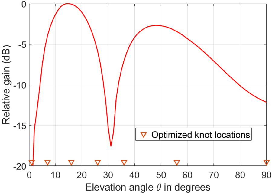
Figure 1: Normalized radiation pattern, $f(\theta )$, of the log-periodic antenna, 4030/LP/10.

The equivalent current distribution on a linear conductor, which would create this radiation pattern, is calculated by solving the following inverse Fourierintegral [2]:

$$I(z^{\prime })=\frac{1}{2\pi }{\int }_{-\mathrm{\infty }}^{\mathrm{\infty }}f(\theta )e^{-j{z}^{\prime }\xi }\mathit{d}\xi ,$$

(21)

where $f(\theta )$ is the radiation pattern, and the variable $\xi =kcos\theta$, and where $k=2\pi /\lambda$ is the wavenumber and $\lambda$ is the wavelength. Furthermore, the antenna is assumed to be located along the vertical $z^{\prime }$ axis, where the prime notation is used to designate the source coordinates.

The knot placement method is applied using $r=7$ distinct knots ($\mathrm{\ell }=6$ intervals) and the increment value $\delta F=1.29$. The optimized knot locations are evaluated at ${\theta }_i=\{0,7,16,26,36,56,90\}$ degrees for $i=1,2,\mathrm{\dots },7$. The CDF, $F(\theta )$, is shown in Fig. 2.

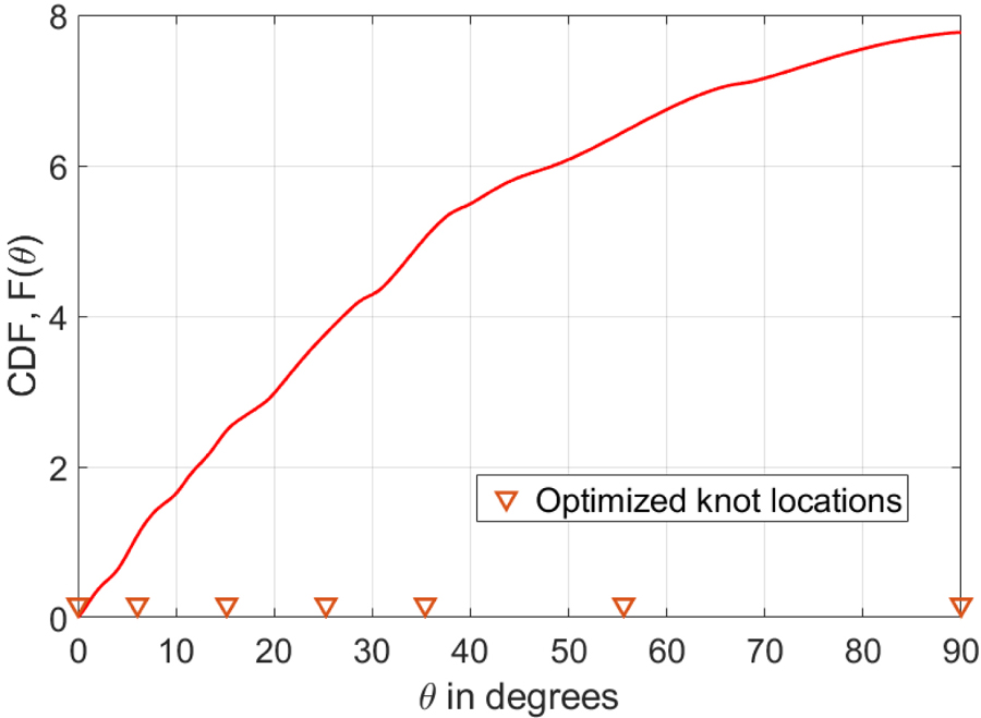
Figure 2: Cumulative distribution function.

The Levin’s method is used to solve the integral in (21) using the optimized knot locations using $n=6$ collocation points for each interval and $m=3$ for the reproducing kernel function as the basis in the collocation formulation. The limits of the integral in (21) are truncated to $\theta \in [{90}^0,0^0]$ or $\xi \in [0,k]$. Thus, the integrals for each sub-interval become:

$$I_j(z^{\prime })=\frac{1}{2\pi }{\int }_{kcos{\theta }_j}^{kcos{\theta }_{j+1}}\dot{f}(\theta )e^{-j{z}^{\prime }\xi }\mathit{d}\xi ,j=1,2,\mathrm{\dots },\mathrm{\ell },$$

(22)

where $\dot{f}(\theta )$ is the part of the radiation pattern in the given interval. Due to the linearity, the total current can be written as:

$$I(z^{\prime })=\sum _{j=1}^{\mathrm{\ell }}{I}_j(z^{\prime }),j=1,2,\mathrm{\dots },\mathrm{\ell }.$$

(23)

The resulting current distribution is shown in Fig. 3.

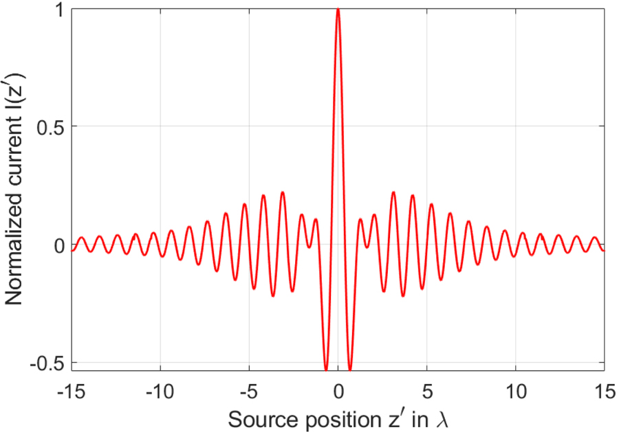
Figure 3: Current distribution along the $z^{\prime }$ axis in terms of the wavelength.

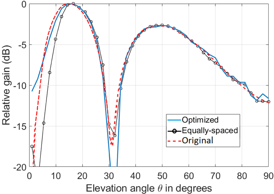
Figure 4: Comparison of the radiation patterns for the knot optimized and the equally spaced Levin’s method ($\mathrm{\ell }=6$, $n=6$).

Table 1: Error and stability analysis in terms of the absolute errors and the matrix condition numbers for the standard (Std.) and the optimized (Opt.) methods

$\mathrm{\ell }$	n	m (RKF)	Error (Std.)	Error (Opt.)	Cond. Num. (Std.)	Cond. Num. (Opt.)
3	3	3	3.00	3.80	2e03	3e07
3	6	3	3.78	2.60	2e06	3e10
3	11	3	3.46	2.70	2e10	2e12
6	3	3	1.97	1.13	5e07	4e11
6	6	3	1.88	1.01	4e10	8e13
6	11	3	1.69	1.36	4e12	6e14
12	3	2	0.90	0.64	7e05	6e06
12	6	2	0.50	0.46	5e07	4e08
12	11	2	0.50	0.47	6e09	4e09

In order to analyze the accuracy of the proposed method, the radiation pattern created by this current distribution must be obtained. This is accomplished by solving the following Fourier integral:

$$f(\theta )={\int }_{-l/2}^{l/2}I(z^{\prime })e^{j\xi z^{\prime }}\mathit{d}{z}^{\prime }={\int }_{-15\lambda }^{15\lambda }I(z^{\prime })e^{jkcos(\theta )z^{\prime }}\mathit{d}{z}^{\prime }.$$

(24)

The Levin’s method is re-used to solve this integral with $r=91$ knots ($\mathrm{\ell }=90$ intervals) and 3 evaluation points ($n=3)$ for each sub-interval for the purpose of obtaining higher accuracy.

The radiation patterns for the optimized knot placement and the equally spaced knot placement methods are compared with the original pattern. The results are shown in Fig. 4. It can be observed that the absolute error is minimized for the proposed optimized knot placement method to be 1.01, whereas for the same settings ($\mathrm{\ell }=6$, $n=6$, $m=3$), the absolute error is 1.88 for the equally spaced knot placement method.

The error and stability analysis results are listed in terms of the absolute errors and the condition numbers of the solution matrices in Table 1 for different $\mathrm{\ell }$ and $n$ values. In a linear equation system, the matrix condition number measures how sensitive the output vector is against the changes in the input vector. These results show that the optimized knot placement method yields more accuracy and slightly less stability than the standard method (equally spaced knot placement) for every $m$ value of the reproducing kernel function.

B. Example 2

In this example, an array antenna is used with a narrow beam radiation at $\theta ={30}^{\circ }$ on the elevation plane (E-plane). The radiation data is transferred into Matlab using B-spline interpolation at 91 points as before, and the resulting pattern function is shown in Fig. 5.

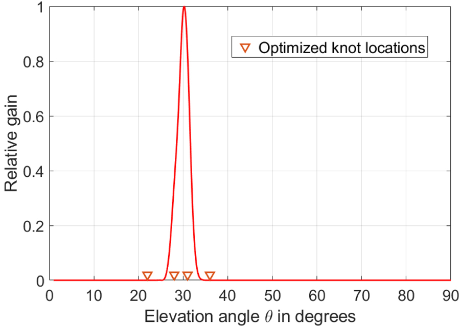
Figure 5: Normalized radiation pattern of the array antenna.

The knot optimization algorithm is carried out for $r=4$ knots ($\mathrm{\ell }=3$ intervals), and the knot locations are obtained at ${\theta }_i=\{27,29,32,34\}$ degrees for $i=1,2,\mathrm{\dots },4$. The cumulative distribution function corresponding to the antenna radiation pattern, $F(\theta )$, is shown in Fig. 6.

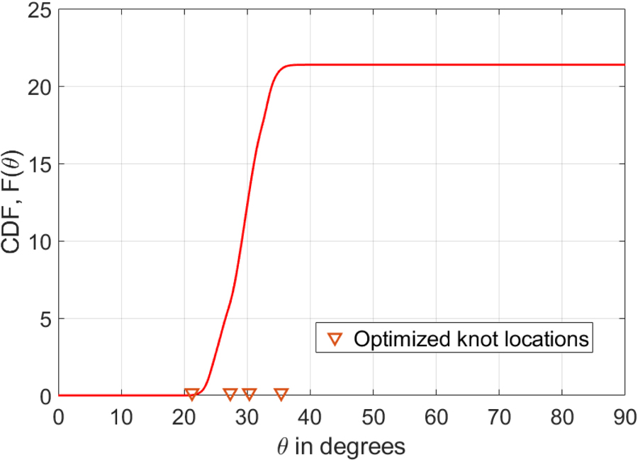
Figure 6: Cumulative distribution function.

Equivalent current distribution on a linear conductor is obtained by using the Levin’s method with optimized knot locations. The resulting current distribution is shown in Fig. 7. The comparison results of the radiation patterns for the knot optimized and the standard methods are shown in Fig. 8. It is observed that the absolute error for the proposed method is 0.16, whereas for the same settings ($\mathrm{\ell }=3$, $n=3$, $m=3$), the absolute error is 2.7 for the equally spaced knot placement method.

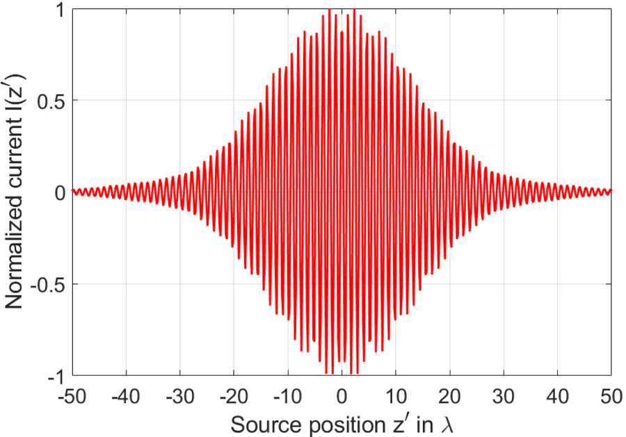
Figure 7: Current distribution along the $z^{\prime }$ axis in terms of the wavelength.

Table 2: Error and stability analysis in terms of the absolute errors and the matrix condition numbers for the standard (Std.) and the optimized (Opt.)methods

$\mathrm{\ell }$	n	m (RKF)	Error (Std.)	Error (Opt.)	Cond. Num. (Std.)	Cond. Num. (Opt.)
3	3	3	2.70	0.16	3e04	3e07
3	6	3	1.50	0.29	3e09	7e11
3	11	3	1.00	1.50	3e11	9e13
6	3	3	4.50	0.46	1e06	1e06
6	6	3	1.38	0.10	2e08	2e08
6	11	3	0.98	0.06	3e09	3e09
12	3	2	6.20	0.15	3e04	6e06
12	6	2	5.00	0.06	3e06	8e08
12	11	2	5.97	0.01	6e07	2e10

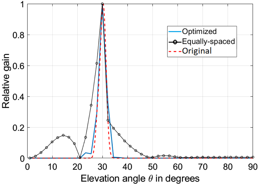
Figure 8: Comparison of the radiation patterns for the knot optimized and the equally spaced Levin’s methods using $\mathrm{\ell }=3$ intervals and $n=3$ collocation points.

The error and stability analysis results are listed for the standard and the optimized methods in Table 2. The results show that the proposed method provides even more significant error reduction.

VI. CONCLUSION

Based on the simulation results, the Levin’s method gives more accurate results when combined with the knot optimization algorithm for antenna synthesis applications. This accuracy improvement can be observed from Table 1 and Table 2, where the error is reduced for the increasing number of intervals ($\mathrm{\ell }$) independent of the number of collocation points ($n$) used for each interval.

The proposed method is particularly advantageous for radiation patterns with small beam widths, as this requires a large number of intervals for the standard technique. This result can be seen from the error analysis between the standard and the proposed techniques in Table 2.

In both examples, the optimized method gives the most accurate result for $m=2$ of the reproducing kernel function, especially with an increase in intervals. For the other $m$ values not listed in Tables 1 and 2, the error is almost the same for different values of m for $n=3$ and degrades significantly for $n>3$, independent of the number of intervals $\mathrm{\ell }$ for both the standard and the optimized methods. Also, the matrix condition number increases with increasing m regardless of the values for $n$ and $\mathrm{\ell }$.

The only drawback of the proposed method is the increased condition number of the solution matrix, which implies that the method’s stability decreases slightly compared to the equal-interval integration technique.

REFERENCES

[1] C. A. Balanis, Antenna Theory, Analysis and Design, New York, John Wiley and Sons, 1997.

[2] W. L. Stutzman and A. T. Gary, Antenna Theory and Design, New Jersey, John Wiley and Sons, 2013.

[3] S. Khan, S. Zaman, A. Arama, and M. Arshad, “On the evaluation of highly oscillatory integrals with high frequency,” Engineering Analysis with Boundary Elements, vol. 121, pp. 116-125, 2020.

[4] D. Levin, ‘‘Procedures for computing one and two dimensional integrals of functions with rapid irregular oscillations,” Mathematics of Computation, vol. 38, no. 158, pp. 531-538, 1982.

[5] S. Khan, S. Zaman, M. Arshad, H. Kang, H. H. Shah, and A. Issakhov, “A well-conditioned and efficient Levin method for highly oscillatory integrals with compactly supported radial basis functions,” Engineering Analysis with Boundary Elements, vol. 131, pp. 51-63, 2021.

[6] S. Xiang, “On the Filon and Levin methods for highly oscillatory integral,” Journal of Computational and Applied Mathematics, vol. 208, pp. 434-439, 2007.

[7] A. Molabahrami, “Galerkin–Levin method for highly oscillatory integrals,” Journal of Computational and Applied Mathematics, vol. 397, pp. 499-507, 2017.

[8] F. Z. Geng and X. Y. Wu, “Reproducing kernel function-based Filon and Levin methods for solving highly oscillatory integral,” Applied Mathematics and Computation, vol. 397, pp. 125980, 2021.

[9] R. Yeh, Y. S. G. Nashed, T. Peterka, and X. Tricoche, “Fast automatic knot placement method for accurate B-spline curve fitting,” Computer-Aided Design, vol. 128, Art no. 102905, 2020.

[10] L. Wasserman, Function Spaces, Lecture Notes, Department of Statistics and Data Science, Carnegie Mellon University.

[11] O. Baver, Reproducing Kernel Hilbert Spaces, M. S. dissertation, Bilkent University, 2005.

BIOGRAPHIES

Goker Sener was born in 1973. He completed his B.S. degree in Electrical Engineering in 1995 at the Wright State University, Dayton, OH. He completed his M.S. and Ph.D. degrees in Electrical and Electronics Engineering in 2004 and 2011 at Middle East Technical University, Ankara, Turkey. He is currently an Assistant Professor in Cankaya University Electrical-Electronics Engineering department, Ankara, Turkey. His fields of interest are electromagnetic theory and antennas.

ACES JOURNAL, Vol. 38, No. 2, 74–79
doi: 10.13052/2023.ACES.J.380201
© 2023 River Publishers

ABSTRACT

I. INTRODUCTION

II. LEVIN’S METHOD

III. REPRODUCING KERNEL FUNCTIONS

IV. KNOT PLACEMENT METHOD

V. ANTENNA DESIGN EXAMPLES

A. Example 1

B. Example 2

VI. CONCLUSION

REFERENCES

BIOGRAPHIES