Unified Formulation for Evaluation and Visualization of Electric and Magnetic Fields Inside Waveguides and Cavities

Zahid Hasan and Atef Elsherbeni

Department of Electrical Engineering
Colorado School of Mines, Golden, CO 80401, USA
aelsherb@mines.edu

Submitted On: October 4, 2022; Accepted On: August 4, 2023

ABSTRACT

The output of this research is an interactive software package developed to enhance and expedite the design of waveguides and cavity resonators through the computation and visualization of the electric and magnetic field distribution. The software features a user-friendly interface through which users can select one of seven different configurations and specify parameters of their design, such as structure dimensions, transverse electric or magnetic mode, mode numbers, operating frequency, number of points of any of the field components along the x, y, and z axis for rectangular structures, and any 2D plane angles between 0 $^{\circ}$ to 360 $^{\circ}$ for cylindrical structures. Both transverse and longitudinal field components can be visualized in vector, color contour or both. The software makes it easy for users to see how the changes of physical dimensions and operating frequency affect the field distribution. Moreover, the user interface allows users to select how visualizations of the field distribution are generated and displayed. Field distributions can be displayed as static images or video animations using appropriate sequencing of computed field values at different plane cuts. The software provides all necessary warning messages for invalid input parameters. Mathematical expressions of the field components used in this software were derived from the classical solution of the wave equations using the separation of variables technique in cartesian coordinates for rectangular configurations and cylindrical coordinates for all other configurations. Results obtained using this software were validated against values found in the literature for similar types of problems, and results show perfect agreement.

Index Terms: Cavity Resonators, Educational Software, EM Fields, Waveguides.

I. INTRODUCTION

The history of the development of waveguides is more than 100 years old. It was first discovered by George C. Southworth who played an important role in radar system design [1]. An electromagnetic field cannot be seen directly [2], only its effects can be observed. Nowadays, technology is growing faster, and millimeter and sub-millimeter waves applications require a combination of active and passive devices. Usually, waveguide-based transmission lines are preferred in the design of low-loss filters, hybrid couplers, power dividers, antennas, etc. [3]. These applications require microwave devices to operate at higher frequencies (above 100 GHz). For operating at these frequency bands, waveguide size needs to be smaller and tolerance requirements need to be tightened. In medical applications, there is a growing need for wireless sensing systems [4]. Passive wireless sensors such as those used in harsh environmental conditions are generally composed of resonant circuits [5]. Cavity resonators are the most used component in passive wireless sensors. For cavity resonators, EM waves bounce back and forth between the cavity walls which produce field oscillations. Evanescent-mode cavity resonators inherently fulfill the need for high frequency passive wireless sensor applications because the size can be greatly reduced. But, with the growing demand for high speed, smaller size devices that consume less power, conventional manufacturing is becoming more and more challenging every day [6]. To the demands for small size and low-power consumption, microwave engineers must fully understand electromagnetic wave propagation inside waveguides and cavity resonators.

WGC (version 2.1) was developed in 1994 to compute and visualize EM field distribution inside waveguides and cavity resonators using an interactive BASIC language for a personal computer running DOS operating system [7]. The executable code of the software was available for the IBM-PC computer family, but it is no longer useable due to recent changes and advancements in computing technology and operating systems. Several software packages for designing and simulating microwave devices and transmission lines, such as Ansys HFSS, CST, and ADS are being used nowadays. For example, the design and simulation of a coplanar and air-gap waveguide transmission line using ADS has been introduced in [8, 9]. CST studio suite has been used for similar design problem [10, 11, 12] and similarly HFSS as in [13, 14, 15]. These software packages are not only expensive, but they also require substantial memory and computational resources to compute and visualize field components inside such configurations of waveguides and cavities. Other software packages like COCAFIL [16] and XFDTD [17] are available, but they require substantial memory and computational resources. A web application to visualize the field pattern inside waveguide has been recently introduced in [18], but it is limited to waveguides with rectangular and circular cross-sections. The software package introduced here WGC (version 3) aims to overcome those challenges. It allows users to visualize the electric and magnetic field distribution inside several types of waveguides and cavity resonators (rectangular, circular, coaxial, baffle, sectoral, sectoral-coaxial, and baffle-coaxial) almost instantaneously on current PC platform. Advantages of using this software include the ability to model a wide variety of waveguide and cavity resonators, less memory requirements and computation time. WGC (version 3) features a user-friendly interface that makes easy for users to quickly model, compute and generate figures and video animations (using appropriate sequencing of computed field values at different plane cuts) of the EM field distribution within their design structure to assess the performance of their design.

WGC (version 3) allows user to observe the change of electric and magnetic fields distribution for different dimensions of the physical or electrical parameters of the cross-sections at different plane cuts. Also, users do not need to limit their interest in any specific mode of operation or order. They have a lot of flexibility in choosing among shapes, dimensions, mode numbers, plane views (x-y, x-z and y-z). Moreover, this software is capable of generating video animations of field distribution as the view angle and position changes. The code is executable on all modern computer families with installed MATLAB version 2021a and later versions. No internet connectivity is needed to run this software. The package can be downloaded from ACES site, software section.

II. MATHEMATICAL DERIVATION OF FIELD EQUATIONS

The objective of this section is to introduce different configurations of waveguide and cavity resonators used in WGC (version 3). The mathematical expressions of the field components are derived from the classical solution of the wave equation using the separation of variables technique.

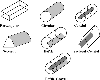
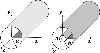
Seven different cross-sections are considered in this software. These are rectangular, circular, sectoral, baffle, coaxial, sectoral coaxial, and baffle coaxial (see Fig. 1). The electromagnetic wave is propagating along the z-axis and the boundary walls are assumed to be perfectly conductive. The waveguides and the cavity resonators are filled with homogeneous, isotropic, and lossless material with permeability denoted by $μ$ and permittivity denoted by $ϵ$ . The field equations for TE and TM modes are obtained after solving the Helmholtz wave equation inside the guide using the separation of variables technique. For rectangular geometry, the Cartesian coordinates system is considered and for the circular, sectoral, baffle, coax, sectoral coax, and baffle coax, the cylindrical coordinates system is used [19].

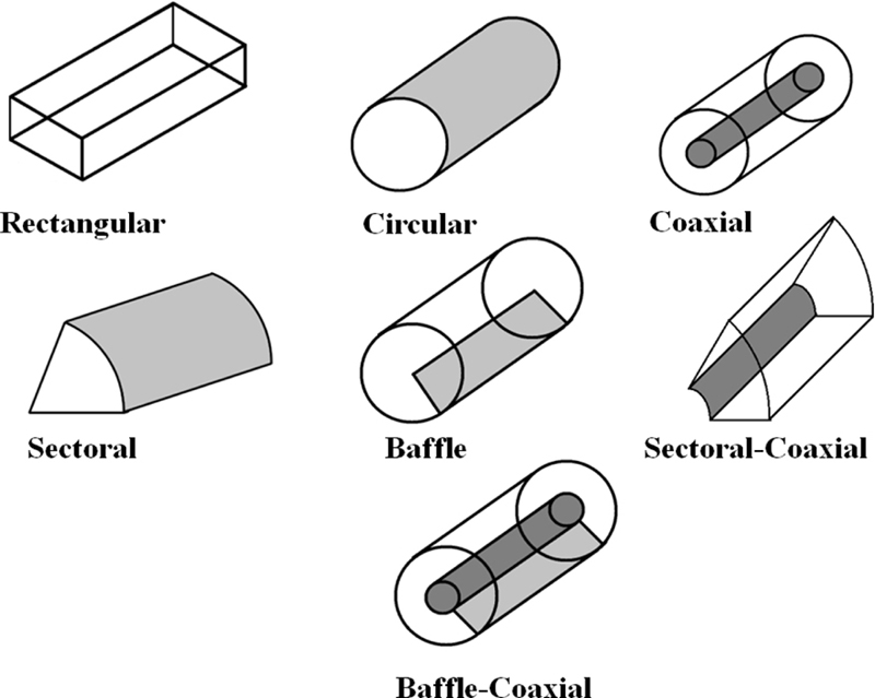
Figure 1: Different cross-sections of waveguides and cavity resonators.

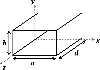
Rectangular Cross-Section: The fields in a rectangular waveguide and cavity resonator consist of several propagating modes which depend on the electrical dimensions, the type, and the position of excitation. Assuming the inner dimensions of the rectangular waveguide are $a$ and $b$ and $d$ along the x, y, and z axes as shown in Fig. 2. A rectangular waveguide supports TM or TE mode but not TEM mode because a hollow rectangular waveguide does not have any inner conductor.

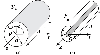
Circular and Coaxial Cross-Section: For the cross-section of circular waveguide and cavity, the radius is denoted by $a$ and for the coaxial cross-section, $a$ is the inner radius and $b$ is the outer radius. The parameter $d$ is the dimension along the propagation of waves as shown in Fig. 3.

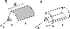
Sectoral and Sectoral-Coaxial Cross-Section: The geometry of sectoral and sectoral-coaxial cross-section are shown in Fig. 4. The only difference is the value of $m$ . For sectoral and sectoral-coaxial cross-section subscript $m$ is a rational number.

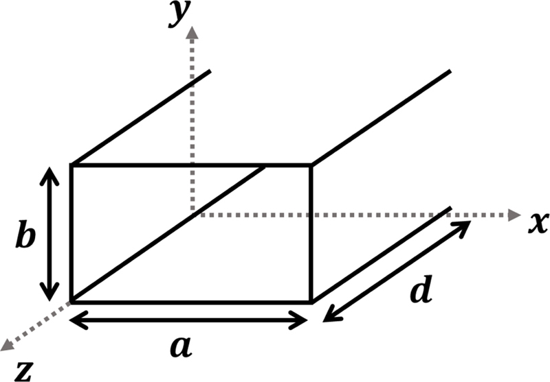
Figure 2: Dimensional parameters of a rectangular waveguide or a cavity.

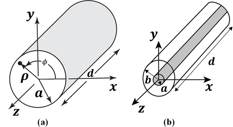
Figure 3: Dimensional parameters of a waveguide or a cavity: (a) circular; (b) coaxial.

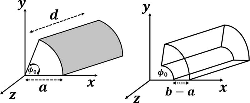
Figure 4: Dimensional parameters of a sectoral and a sectoral-coaxial waveguide or a cavity.

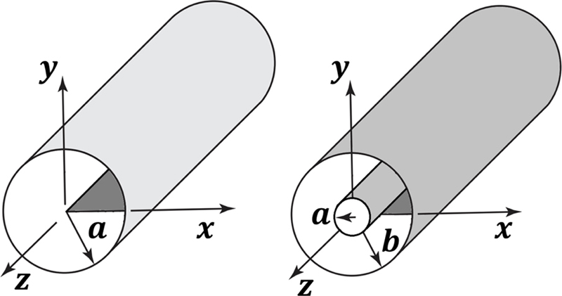
Figure 5: Dimensional parameters of a circular baffle and a baffle-coaxial waveguide or a cavity.

Baffle and Baffle-Coaxial Cross-Section: When a conducting plate is inserted into a hollow cylindrical waveguide or cavity resonator, then the baffle configuration is created (see Fig. 5). The field equations for these configurations are similar to the circular except for the value of $ϕ_{0}$ . For baffle and baffle-coaxial waveguides and cavity resonators $ϕ_{0} = 2 π$ .

III. SOFTWARE DESIGN

This section provides the design configuration of the software which will visually represent the electric and magnetic field distribution inside waveguides and cavity resonators for different modes of operation. The full software package is designed in the MATLAB App designer platform. First, field equations in this document have been verified with existing figures documented in [21, 22]. Then in MATLAB App designer, two windows are created to access the cross-sections of different waveguides and cavity resonators and later seven different windows are designed for seven different configurations of waveguides and cavity resonators.

MATLAB App Designer Platform: App designer helps to design professional apps. Simple drag and drop visual components in the app designer window help to layout the design of the graphical user interface (GUI) and to use the integrated editor to quickly program its behaviour. App designer has two view options, one is design view and another one is code view. In the design view window, one can easily layout the visual components from the component library. Each component has callback options that allow commanding individual components separately. Callback functions allow working in the code view window. Also, the code view window has property, functions, and app input arguments options which give the freedom to work in multiple app window settings. App Designer can automatically check for coding problems using the Code Analyzer. Standalone applications can be created by using MATLAB Compiler and Simulink Compiler to share them royalty-free with other users [20].

Graphical User Interface Development: Our software has nine different windows. The first window is called the main menu which will guide users to the next option menu. There a user can select which cross-section of a waveguide or a cavity they want to select. After that, the user will be able to generate figures or create movies for different modes of operation in a waveguide or a cavity.

Layout and Operation of the Software: The layout of the software is mainly categorized into four main windows. Those are Main Window, Geometry Selection, and Parameters Screen and Output Screen (Figure and Video Creation). Each of them is described below.

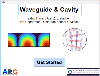
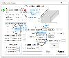
Main Window: The window that will appear when a user starts the software is called the main window (shown in Fig. 6). In this window at the top of the left corner, there is a button called help. If the user selects this button, he/she will find two options there. One is about the app and the other will help the user find the contact details of the authors. In the main window, there is a big button called “Get Started”. When the user presses that button, it will lead to the next geometry selectionwindow.

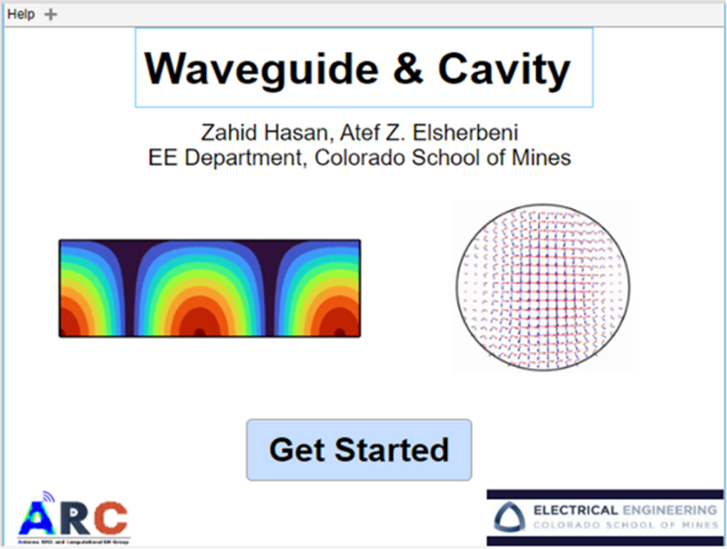
Figure 6: Main window of WGC software.

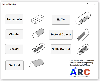
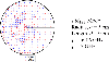
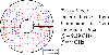
Geometry Selection: The geometry selection (Options Menu) window is shown in Fig. 7. Seven different cross-sections are included. Those are rectangular, circular, sectoral, baffle, coaxial, sectoral-coaxial, baffle-coaxial cross-sections. When the user clicks any button beside a picture, the next window will open the parameters window of this picture geometry, and this geometry selection window will close automatically.

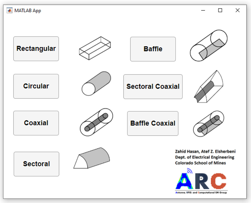
Figure 7: Geometry selection window.

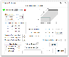
Parameters Screen: The parameters screen window is different for different geometry selections. Each of them has a waveguide or a cavity selection button, mode choice option, input for waveguide and cavity dimensions, operation frequency, and plane cut option. Also, there are cut-off, resonant frequency calculator option which depends on the dimensions of the cross-sections of waveguides and cavity resonators. The waveguide and cavity selection button will enable or disable some options (which are not needed) in the parameter screens. In the waveguide and cavity dimension box, three different units (cm, mm, and inch) are added in the drop-down menu. There is also an input for the number of points along the x, y, and z-axis. It will give the users the flexibility to see the propagation of electromagnetic waves as to how they want to see them. In the bottom of the left corner, there are two options for figure or video creation. Users can save their works as a picture as well as a video. The drop-down menu of the figure or video creation buttons, contains 5 different options. These are vector plot, E-field strength, H-field strength, E-field strength with vector, and H-field strength with vector. At the end of the right corner of the window there are three buttons called “Check”, “Run”, and “Return” buttons. The “Check” button checks all the input parameters. If there is an error in the input parameters, this “Check” button will show warning messages. Also, if the user puts some wrong inputs while trying to find the cut-off and resonance frequency for waveguides or cavity resonators, this “calculate” button will also show some warning messages. Initially, the “Run” button is kept deactivated so that users can easily understand the mistakes if they do any by pressing the “Check” button. If there is no error, the “Run” button will be activated, and the user will be able to see the picture or the video according to his/her options selection. Right below the Create figure and Video box, there is a text area where the user can see the message about the current figure or video creation status. The “Return” button will get the user return back to the geometry selection window to work further with the app. The parameters screen for rectangular cross-section is shown in Fig. 8.

Figures of EM Fields: When the user selects the “Create Figure” button, initially, it is selected for the vector plot. But the user can change the view option by pressing the drop-down menu just beside the button. After creating one figure the user does not need to exit the figure window to see another configuration of input parameters. This will help the user to compare figures by placing them side by side. And after that, the user can save those images in whichever directory they want toselect.

Video Animations of EM Fields: The video creation option is pretty much like the figure creation option. The animation is created using an appropriate sequencing of computed field values at different plane cuts. For creating a video, more time is needed than figure creation. So, at that time a progress bar and successful bar are included so that the user can understand that the video is being created, and it will take some time. When the video creation is completed, a success message will appear and telling the user that the movie creation issuccessful.

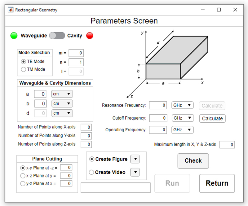
Figure 8: Parameters screen window for rectangular waveguides and cavities.

IV. ILLUSTRATED EXAMPLES

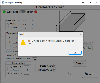
This section provides illustrated examples of software functionality. Each parameters screen has the option to switch between waveguide and cavity. The default position of the switch is for waveguide. When a user slides the switch to cavity, the red light next to it turns green and the green light next to the waveguide turns red. When the user changes the switch position back to waveguide, the light color will change again. This way, a user receives feedback from the software confirming which of the two configurations is active. Figure 9 shows different options and dropdown menus in the parameters screen widow. Initially the “Run” button is disabled. If all inputs are valid, then after clicking the “Check” button no error is shown and that enables the “Run” button. The “Return” button will take users back to the geometry selection window. For invalid inputs, users will be warned by showing error messages. While checking the error, the software automatically disables the “Run” button, and this makes the user understand that some corrections need to be done. Figure 10 shows a warning message for invalid input in the mode number.

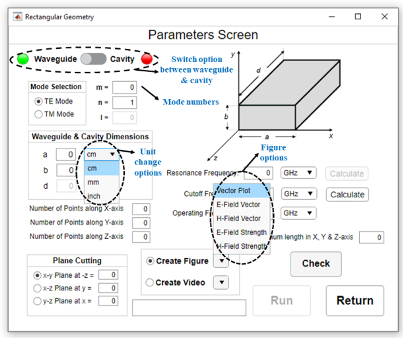
Figure 9: Different options in parameters screen window.

Figures for Waveguide: For valid inputs, some figures of the coaxial and sectoral-coaxial waveguide for different views are shown here in Figs. 11–14.

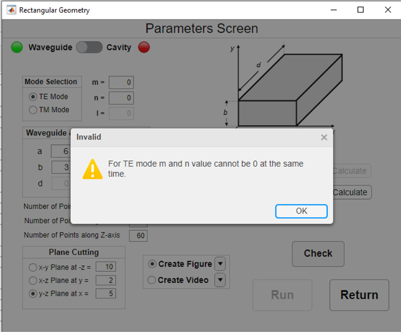
Figure 10: Checking the error message for invalid mode number.

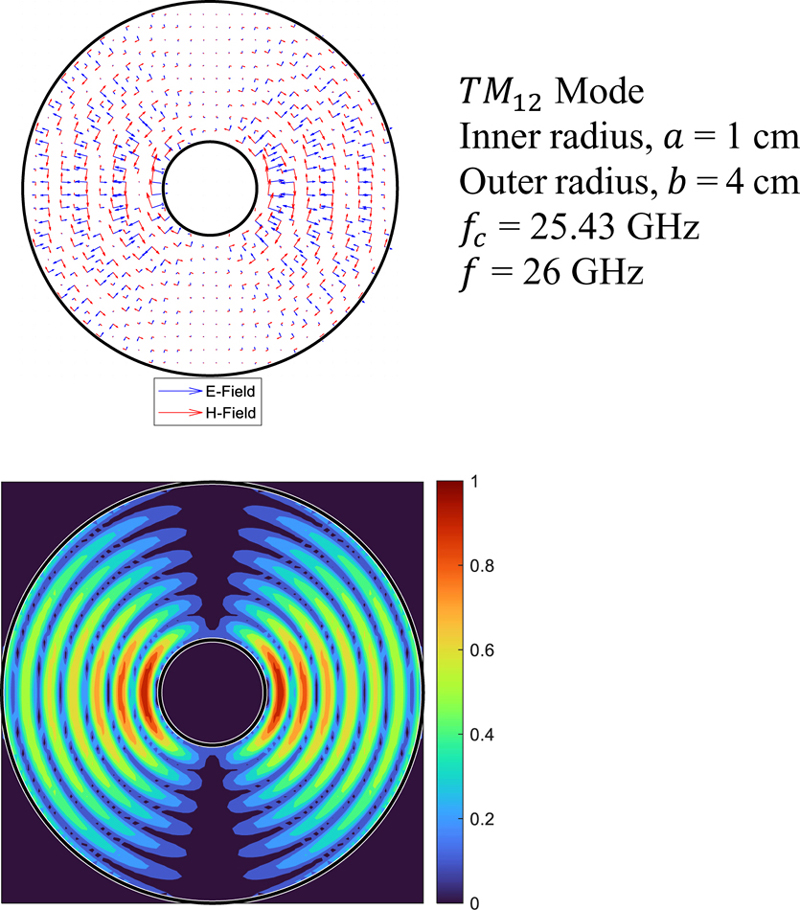
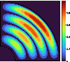
Figure 11: Vector and field strength of E-Field or H-Field for $T M_{12}$ mode of a coaxial waveguide.

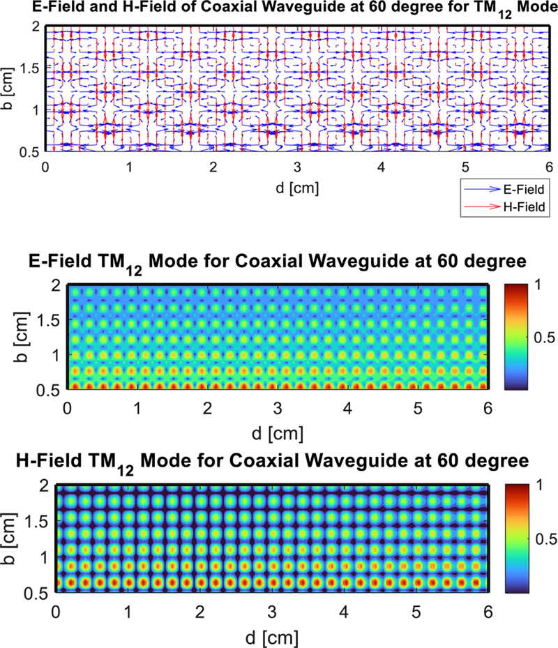
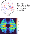
Figure 12: Vectors and field strength for $T M_{12}$ mode in the $60^{^{\circ}}$ plane cut of a coaxial waveguide.

Figures for Cavity: Switching to cavity mode, activates some input parameters in the parameters screen. Those input parameters have no function in the waveguide mode and that is why those are inactive in the waveguide mode. Illustrated examples have been given for baffle and baffle-coaxial cavity as shown inFigs. 15–18.

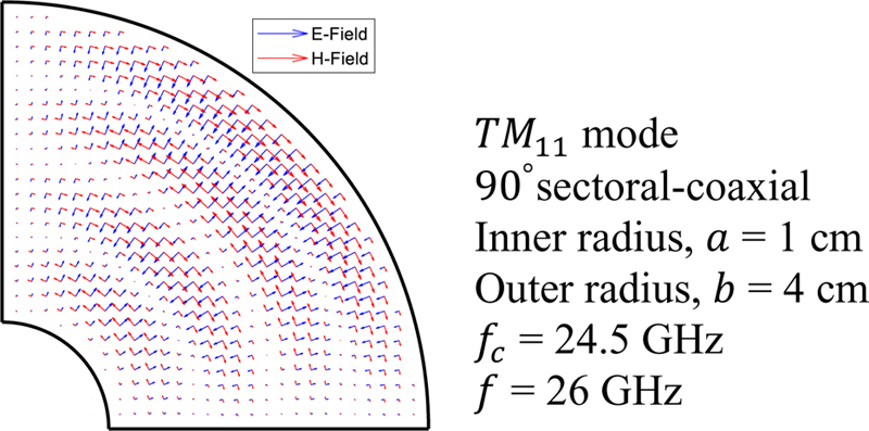
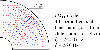
Figure 13: Cross-sectional vector fields for the $T M_{11}$ mode of a $90^{^{\circ}}$ sectoral coaxial waveguide.

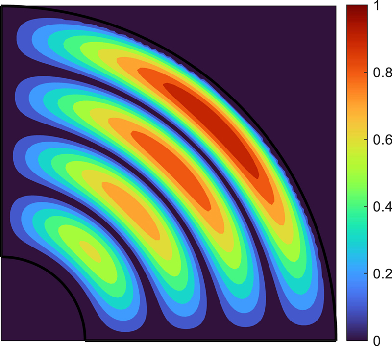
Figure 14: E-Field and H-Field strength at the cross-section of a $90^{^{\circ}}$ sectoral coaxial waveguide for $T M_{11}$ mode.

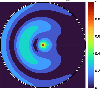
Figure 15: Cross-sectional vector fields for the $T M_{122}$ mode of a baffle cavity.

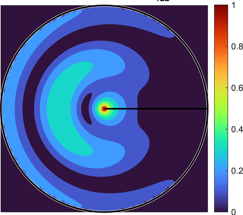
Figure 16: E-Field and H-Field strength at the cross-section of a baffle cavity for $T M_{122}$ mode.

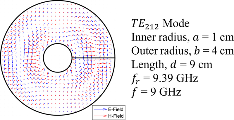
Figure 17: Cross-sectional vector fields for the $T E_{212}$ mode of a baffle-coaxial cavity.

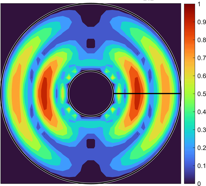
Figure 18: E-Field and H-Field strength at the cross-section of a baffle-coaxial cavity for $T E_{212}$ mode.

This section provided illustrated examples (Figs. 11–18) for various cross-sections of waveguide and cavity resonator configurations. For rectangular cross-section, users can view the field pattern in x-y, x-z and y-z axis. For cylindrical cross-sections, users can view field distribution in x-y axis and in any arbitrary angle between $0^{^{\circ}}$ and $360^{^{\circ}}$ . However, since the sectoral cross-sections limits the geometry structure with the angle $ϕ_{0}$ , users can observe field pattern between $0^{^{\circ}}$ and $ϕ_{0}$ degrees. If users input in the view angle is greater than the sectoral angle $ϕ_{0}$ , for sectoral and sectoral-coaxial cross-sections, WGC will show warningmessages.

V. CONCLUSION

Coding languages used to build WGC (version 2.1) are no longer available and the major advanced in computer technology, rendered the software unusable. This research is the rework and major update of the waveguide and cavity software (WGC version 2.1). The revival of the software was essential to compute and visualize the electric and magnetic fields inside waveguides and cavity resonators on current computing platforms. Several enhancements were made to make the software more powerful and user-friendly.

The software package presented in this paper WGC (version 3) has been developed in the MATLAB App designer platform. WGC’s graphical user interface (GUI) is easy to use and self-explanatory. The main window provides information about the software and the contact info of the authors. Users are able to select one of the seven cross-sections listed by names along with graphical representation. Based on selected cross-section, the appropriate parameters screen is displayed to allow the user to enter physical dimensions, operating frequency and select how to visualize the results. Warning messages are generated for invalid input parameters. WGC allows users to save the computed field values for comparison and validation against theoretical calculations and measurements.

Performance evaluation of WGC through comparisons with HFSS and CST’s computational time and memory requirements for similar waveguides and cavity resonators problem, may be conducted for benchmarking purposes. Future work also includes research on the development of mathematical expressions for dielectric, partially filled, and rigid waveguides and cavity resonators for inclusion as modelling options in thesoftware.

REFERENCES

[1] K. S. Packard, “The origin of waveguides: A case of multiple rediscovery,” IEEE Transactions on Microwave Theory and Techniques, vol. 32, no. 9, pp. 961-969, 1984.

[2] N. N. Rao, “PC-assisted instruction of introductory electromagnetics,” IEEE Transactions on Education, vol. 33, no. 1, pp. 51-59, 1990.

[3] S. Farjana, M. Ghaderi, A. U. Zaman, S. Rahiminejad, P. Lundgren, and P. Enoksson, “Low-loss gap waveguide transmission line and transitions at 220–320 GHz using dry film micromachining,” IEEE Transactions on Components, Packaging and Manufacturing Technology, vol. 11, no. 11, pp. 2012-2021, 2021.

[4] REMCOM, “How to build a rectangular waveguide in XFDTD,” Remcom Inc State College, PA, [Online].

[5] Y. Zhao, Y. Li, B. Pan, S. H. Kim, Z. Liu, M. M. Tentzeris, J. Papapolymerou, and M. G. Allen, “RF evanescent-mode cavity resonator for passive wireless sensor applications,” Sensors and Actuators A: Physical, vol. 161, no. 1-2, pp. 322-328,2010.

[6] A. Sahu, V. K. Devabhaktuni, R. K. Mishra, and P. H. Aaen, “Recent advances in theory and applications of substrate-integrated waveguides: a review,” International Journal of RF and Microwave Computer-Aided Engineering, vol. 26, no. 2, pp. 129-145, 2016.

[7] A. Z. Elsherbeni and C. D. Taylor, “Interactive visualizations of electromagnetic fields inside waveguides and cavity resonators using the WGC program,” Computer Applications in Engineering Education, vol. 2, no. 2, pp. 97-107,1994.

[8] F. D. Mbairi and H. Hesselbom, “High frequency design and characterization of SU-8 based conductor backed coplanar waveguide transmission lines,” in Proceedings. International Symposium on Advanced Packaging Materials: Processes, Properties and Interfaces, 2005, pp. 243-248,2005.

[9] I. Jeong, S. H. Shin, J. H. Go, J. S. Lee, C. M. Nam, D. W. Kim, and Y. S. Kwon, “High-performance air-gap transmission lines and inductors for millimeter-wave applications,” IEEE Transactions on Microwave Theory and Techniques, vol. 50, no. 12, pp. 2850-2855, 2002.

[10] F. Taringou, D. Dousset, J. Bornemann, and K. Wu, “Substrate-integrated waveguide transitions to planar transmission-line technologies,” in 2012 IEEE/MTT-S International Microwave Symposium Digest, pp. 1-3, 2012.

[11] J. Shi, H. Chen, S. Zheng, D. Li, R. Rimmer, and H. Wang, “Comparison of measured and calculated coupling between a waveguide and an RF cavity using CST microwave studio,” Thomas Jefferson National Accelerator Facility, Newport News, VA, technical report, 2006.

[12] E. Pucci, A. U. Zaman, E. Rajo-Iglesias, P.-S. Kildal, and A. Kishk, “Losses in ridge gap waveguide compared with rectangular waveguides and microstrip transmission lines,” in Proceedings of the Fourth European Conference on Antennas and Propagation, pp. 1-4,2010.

[13] N. A. Amoli, S. Sivapurapu, R. Chen, Y. Zhou, M. L. Bellaredj, P. A. Kohl, S. K. Sitaraman, and M. Swaminathan, “Screen-printed flexible coplanar waveguide transmission lines: Multi-physics modeling and measurement,” in 2019 IEEE 69th Electronic Components and Technology Conference (ECTC), pp. 249-257,2019.

[14] S. H. Kamath, R. Arora, and V. Agarwal, “Studying the characteristics of a rectangular waveguide using HFSS,” International Journal of Computer Applications, vol. 118, no. 21, pp. 5-8,2015.

[15] Y. Zhou, H. Liu, E. Li, G. Guo, and T. Yang, “Design of a wideband transition from double-ridge waveguide to microstrip line,” International Conference on Microwave and Millimeter Wave Technology, pp. 737-740, 2010.

[16] Zeland Software Inc., Fremont, CA, “Software for optimizing the design and low-cost production of waveguide filters,” Microwave Journal, [Accessed: March 24, 2022]: https://www.microwavejournal.com, 2002.

[17] M. Al Ameen, J. Liu, and K. Kwak, “Security and privacy issues in wireless sensor networks for healthcare applications,” Journal of medical systems, vol. 36, no. 1, pp. 93-101,2012.

[18] S. Mitheran, R. T. Narayanan, and R. Singaravelu, “User-friendly waveguide mode visualizer, Educator’s corner,” IEEE Microwave Magazine, vol. 23, no. 5, pp. 96-100, 2022.

[19] A. Z. Elsherbeni and C. D. Taylor, Jr., “Electromagnetic Fields Inside Waveguides and cavity resonators; WGC (version 2.1),” Software Book II, Center on Computer Applications for Electromagnetic Education (CAEME), 1994.

[20] MathWorks, “App designer-create desktop and web apps in MATLAB,” Mathworks Natick, MA, https://www.mathworks.com [Accessed: August 01, 2021].

[21] C. A. Balanis, Advanced Engineering Electromagnetics. John Wiley & Sons, 2012.

[22] A. Elsherbeni, D. Kajfez, and S. Zeng, “Circular sectoral waveguides,” IEEE Antennas and Propagation Magazine, vol. 33, no. 6, pp. 20-27,1991.

BIOGRAPHIES

Zahid Hasan completed his B.Sc. and M.Sc. from the Department of Electrical and Electronic Engineering at University of Dhaka, Bangladesh. He earned his second master’s degree in the Electrical Engineering department of Colorado School of Mines. He was employed as a teaching assistant there and a member of the ARC Research Group directed by Dr. Atef Elsherbeni.

Currently, he is pursuing his Ph.D. degree at the Electrical and Computer Engineering department at University of Central Florida. At the first year of his Ph.D., he was awarded the ORCGS Doctoral Fellowship at UCF. He is also employed as a research assistant and a member of the ARMI Research Group directed by Dr. Xun Gong. Besides, he is serving as a secretary in the IEEE AP/MTT chapter in Orlando.

Atef Z. Elsherbeni received an honor B.Sc. degree in electronics and communications, an honor B.Sc. degree in applied physics, and a M.Eng. degree in electrical engineering, all from Cairo University, Cairo, Egypt, in 1976, 1979, and 1982, respectively, and a Ph.D. degree in electrical engineering from Manitoba University, Winnipeg, Manitoba, Canada, in 1987. He started his engineering career as a part-time software and system design engineer from March 1980 to December 1982 at the Automated Data System Center, Cairo, Egypt. From January to August 1987, he was a post-doctoral fellow at Manitoba University. Dr. Elsherbeni joined the faculty at the University of Mississippi in August 1987 as an assistant professor of electrical engineering. He advanced to the rank of associate professor in July 1991, and to the rank of professor in July 1997. He was the associate dean of the college of Engineering for Research and Graduate Programs from July 2009 to July 2013 at the University of Mississippi. He then joined the Electrical Engineering and Computer Science (EECS) Department at Colorado School of Mines in August 2013 as the Dobelman Distinguished Chair Professor. He was appointed the interim department head for (EECS) from 2015 to 2016, and from 2016 to 2018 he was the Electrical Engineering Department head. He spent a sabbatical term in 1996 at the Electrical Engineering Department, University of California at Los Angeles (UCLA) and was a visiting professor at Magdeburg University during the summer of 2005 and at Tampere University of Technology in Finland during the summer of 2007. In 2009 he was selected as Finland Distinguished Professor by the Academy of Finland and TEKES.

Over the years, Dr. Elsherbeni participated in acquiring millions of dollars to support his research group activities dealing with scattering and diffraction of EM waves by dielectric and metal objects, finite difference time domain analysis of antennas and microwave devices, field visualization and software development for EM education, interactions of electromagnetic waves with the human body, RFID and sensor integrated RFID systems, reflector and printed antennas and antenna arrays for radars, UAV, and personal communication systems, antennas for wideband applications, and measurements of antenna characteristics and material properties. Dr. Elsherbeni is an IEEE life fellow and ACES fellow. He is the editor-in-chief for ACES Journal, and a past associate editor to the Radio Science journal. He was the chair of the Engineering and Physics Division of the Mississippi Academy of Science, the chair of the Educational Activity Committee for IEEE Region 3 Section, and the general chair for the 2014 APS-URSI Symposium and the president of ACES Society from 2013 to 2015. Dr. Elsherbeni is selected as distinguished lecturer for IEEE Antennas and Propagation Society for 2020-2023.