Optimal Antenna Pattern Design for the Instantaneous MIMO Channel

Cuicui Zhang, Shuo Wang, Ming Zhang, Xiaobo Liu, and Anxue Zhang

School of Information and Communications Engineering
Xi’an Jiaotong University, Xi’an, 710049, China
anxuezhang@mail.xjtu.edu.cn

Submitted On: October 29, 2022; Accepted On: January 13, 2023

ABSTRACT

Due to the rapid attenuation of the millimeter wave, it is necessary to use very large-scale antenna arrays in millimeter wave communications to get ultra-high directivity which improves the transmission distance and the signal-to-noise ratio. Considering the cost of large-scale RF links, analog beamforming plays an important role in large-scale MIMO communications. This paper discusses the calculation method of the antenna pattern that best matches the instantaneous MIMO channel in analog beamforming. By giving piecewise modeling on the antenna pattern, singular value decomposition and the water-filling algorithm are used to obtain the antenna pattern and the power distribution among antennas. The optimal antenna pattern can provide the target pattern for antenna synthesis to get the maximum capacity. The simulation results show that the method is effective.

Index Terms: maximum capacity, MIMO, optimal antenna pattern, spatial cluster model.

I. INTRODUCTION

With commercial use of the 5th generation mobile communication technology and the layout of 6th generation mobile communication technology, the communication system is developing toward ultra-large bandwidth and ultra-low delay. Ultra-large-scale antenna technology and millimeter wave communication have received extensive attention [1-4]. Due to the rapid attenuation of the millimeter wave, beamforming technology of very large-scale antenna arrays is proposed [5]. Considering the high cost of large-scale RF links, analog beamforming plays an important role in large-scale MIMO communications. Analog beamforming based on the statistical channel model has been used to guide antenna design [6-8]. There is also hybrid beamforming based on new antenna structures [9], including hybrid beamforming on smart antennas [10], reconfigurable intelligent surface antennas [11, 12], and holographic antennas [13, 14].

However, the above methods use models in which the antenna parameters are included in the performance measurement of the communication system. The antenna design parameters are obtained first through optimization algorithms and then the antenna pattern is obtained indirectly. All these methods require the designers to have knowledge both in antenna and communication fields, and different antenna structures need to be remodeled and reanalyzed, and the algorithm complexity is high.

Due to the cluster sparsity of millimeter wave channels, the complexity of beamforming methods using the deterministic and semi-deterministic spatial cluster channel model is reduced. In this paper, for the instantaneous MIMO channel which is modeled by the spatial cluster channel model, the antenna pattern best matching the wireless propagation environment is directly obtained. Without the antenna parameters involved, only the piecewise modeling and power constraints of the antenna pattern are carried out. The closed-form of the optimal antenna pattern can be obtained by using singular value decomposition. The optimal pattern can be used as the target pattern in antenna synthesis methods, such as the genetic algorithm [15], particle swarm optimization algorithm [16, 17], and other intelligence algorithms [18, 19], to further obtain the antenna parameters.

Antenna mutual coupling is a very important parameter that will greatly affect the performance of a tight array. There is literature on how to reduce mutual coupling in MIMO systems [20, 21]. In this paper, the antenna spacing is set to half wavelength, when the effect of mutual coupling is small. To focus on the optimal pattern design, the mutual coupling is not considered in this paper. It will be considered in further work.

II. OPTIMAL ANTENNA DESIGN OF MIMO-SU

TR 38.901 [22] studies a channel model for frequencies from 0.5 to 100 GHz in the fifth generation mobile communication system. It is widely used in the research in the communication field. According to the channel description in 3GPP TR 38.901 [22], the antenna radiation characteristic is an important factor of the wireless channel. The antenna radiation characteristic and the wireless propagation environment jointly determine the wireless channel [23]. If the wireless propagation environment is full rank, such as a rich multi-path environment, the rank loss of the antenna radiation characteristic will lead to rank loss of the transmission channel, which will result in the reduction of the multiplexing gain. On the contrary, a suitable antenna radiation characteristic not only ensures the full rank of the transmission channel but also has a good condition number in terms of diversity gain and multiplexing gain [24]. Therefore, it is valuable to find out the most suitable antenna pattern for the wireless propagation environment.

A. System model

3GPP TR 38.901 is the specification that studies on channel model for frequencies from 0.5 to 100 GHz use, in which the channel is modeled as some spatial clusters. The channel coefficients without polarization in consideration are given by (1) when the transmitting antenna array and receiving antenna array are both linear arrays, and both aligned with the x-axis, as shown in Fig. 1.

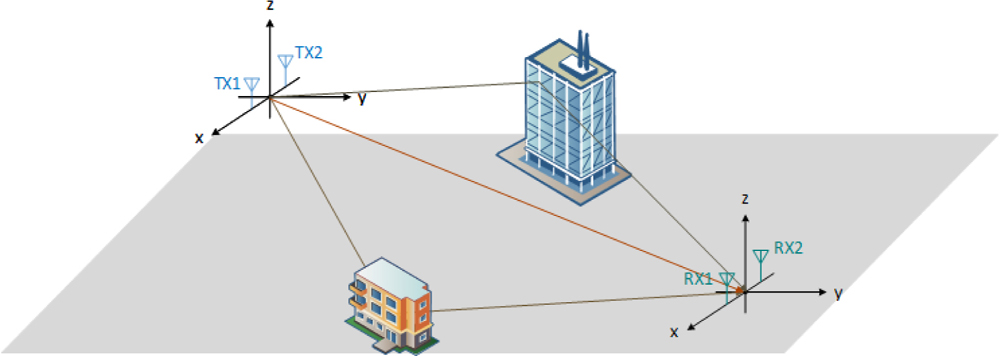
Figure 1: Channel with 3 clusters.

$H_{m,k}=$	${\displaystyle {\sum }_{n=1}^N}(h_{n}f{r}_m(Ao{A}_n,Zo{A}_n)*f{t}_k(Ao{D}_n,Zo{D}_n)$
$*e^{j\left(m-1\right)*\kappa d_r*cos\left(Ao{A}_n\right)cos\left(Zo{A}_n\right)}$
$*e^{j\left(k-1\right)*\kappa d_t*cos\left(Ao{D}_n\right)cos\left(Zo{D}_n\right)}),$	(1. a)
$${\alpha }_n=\kappa d_r*\cos \left(Ao{A}_n\right)*\cos (Zo{A}_n),$$	(1. b)
$${\beta }_n=\kappa d_t*\cos \left(Ao{D}_n\right)*\cos \left(Zo{D}_n\right).$$	(1. c)

The channel coefficients can be written in matrix form (2), which is shown at the bottom of this page, where K and M are the numbers of transmitting and receiving antennas and N is the number of clusters. ${\alpha }_n$ is the phase difference caused by the nth cluster on two adjacent receiving antennas, ${\beta }_n$ is the phase difference caused by the nth cluster on two adjacent transmitting antennas. $f_{t_k}(\theta ,\phi )$ is the kth Tx antenna pattern. $f_{r_m}(\theta ,\phi )$ is the mth Rx antenna pattern. ${\tilde{H}}_{M\times N}$ shows the joint effect of the wireless propagation environment and the receiving antenna on the channel. $F_{N\times K}$ shows the effect of the directivity of the transmission antenna on the channel.

Assuming that the receiving antenna is omnidirectional, the numbers of transmitting and receiving antennas are both 2, the antenna spacing is half a wavelength, and the propagation environment has 3 clusters as shown in Fig. 1, then the channel matrix H is given by (3), which is shown on the next page.

B. Problem formulation

The capacity for MIMO channels is given by (4), [25].

$\mathrm{C}$	$={\log }_2\det (I_M+{\displaystyle \frac{P}{{\sigma }^2}}{H}_{M\times K}*R_{ss}*H_{M\times K}{}^H)$
$={\log }_2\det (I_M+{\displaystyle \frac{P}{{\sigma }^2}}{\tilde{H}}_{M\times N}*F_{N\times K}*R_{ss}*F^H{}_{K\times N}*\tilde{H}^H{}_{N\times M}),$	(4. a)
$$R_{ss}=\left[\begin{array}{ccc}\hfill p_1\hfill & \hfill \mathrm{\dots }\hfill & \hfill 0\hfill \\ \hfill \mathrm{⋮}\hfill & \hfill \mathrm{\ddots }\hfill & \hfill \mathrm{⋮}\hfill \\ \hfill 0\hfill & \hfill \mathrm{\dots }\hfill & \hfill p_K\hfill \end{array}\right],$$	(4. b)

where $R_{ss}$ is the covariance matrix of the transmission data streams, representing the transmission power distribution. The normalized $p_k$ satisfies,

$${\sum }_k{p}_k=1,$$

(5)

the optimal antenna pattern can be obtained by the following optimization problem,

$$\underset{(F,R_{ss})}{maximize}C,$$

(6. a)

subject to

$$Tr\left(R_{ss}\right)=1.$$

(6. b)

To solve the above problem, the power constraint of $R_{ss}$ is not enough, the constraint about the antenna pattern matrix F is needed too. The antenna pattern matrix F needs to be modeled first.

$H_{2\times 2}$	$=\left[\begin{array}{ccc}\hfill h_1\hfill & \hfill h_2\hfill & \hfill h_3\hfill \\ \hfill h_1{e}^{j\pi *\cos \left(Ao{A}_1\right)*\cos \left(Zo{A}_1\right)}\hfill & \hfill h_2{e}^{j\pi *\cos \left(Ao{A}_2\right)*\cos \left(Zo{A}_2\right)}\hfill & \hfill h_3{e}^{j\pi *\cos \left(Ao{A}_3\right)*\cos \left(Zo{A}_3\right)}\hfill \end{array}\right]*$
$\left[\begin{array}{cc}\hfill f_{t_1}(Ao{D}_1,Zo{D}_1)\hfill & \hfill f_{t_2}(Ao{D}_1,Zo{D}_1)e^{j\pi *\cos \left(Ao{D}_1\right)*\cos (Zo{D}_1)}\hfill \\ \hfill f_{t_1}(Ao{D}_2,Zo{D}_2)\hfill & \hfill f_{t_2}(Ao{D}_2,Zo{D}_2)e^{j\pi *\cos \left(Ao{D}_2\right)*\cos (Zo{D}_2)}\hfill \\ \hfill f_{t_1}(Ao{D}_3,Zo{D}_3)\hfill & \hfill f_{t_2}(Ao{D}_3,Zo{D}_3)e^{j\pi *\cos \left(Ao{D}_3\right)*\cos (Zo{D}_3)}\hfill \end{array}\right].$	(3)
$H_{M\times K}$	$=\left[\begin{array}{ccc}\hfill \begin{array}{cc}\hfill \begin{array}{c}\hfill h_1{f}_{r_1}(Ao{A}_1,Zo{A}_1)\hfill \\ \hfill h_1{f}_{r_2}(Ao{A}_1,Zo{A}_1)e^{j{\alpha }_1}\hfill \end{array}\hfill & \hfill \begin{array}{c}\hfill h_2{f}_{r_1}(Ao{A}_2,Zo{A}_2)\hfill \\ \hfill h_2{f}_{r_2}(Ao{A}_2,Zo{A}_2)e^{j{\alpha }_2}\hfill \end{array}\hfill \end{array}\hfill & \hfill \begin{array}{c}\hfill \mathrm{\cdots }\hfill \\ \hfill \mathrm{\cdots }\hfill \end{array}\hfill & \hfill \begin{array}{c}\hfill h_N{f}_{r_1}(Ao{A}_N,Zo{A}_N)\hfill \\ \hfill h_N{f}_{r_2}(Ao{A}_N,Zo{A}_N)e^{j{\alpha }_N}\hfill \end{array}\hfill \\ \hfill \begin{array}{cc}\hfill \mathrm{⋮}\hfill & \hfill \mathrm{⋮}\hfill \end{array}\hfill & \hfill \mathrm{\ddots }\hfill & \hfill \mathrm{⋮}\hfill \\ \hfill \begin{array}{cc}\hfill h_1{f}_{r_M}(Ao{A}_1,Zo{A}_1)e^{j\left(M-1\right){\alpha }_1}\hfill & \hfill h_2{f}_{r_M}(Ao{A}_2,Zo{A}_2)e^{j\left(M-1\right){\alpha }_2}\hfill \end{array}\hfill & \hfill \mathrm{\cdots }\hfill & \hfill h_N{f}_{r_M}(Ao{A}_N,Zo{A}_N)e^{j\left(M-1\right){\alpha }_N}\hfill \end{array}\right]*$
$\left[\begin{array}{ccc}\hfill \begin{array}{cc}\hfill \begin{array}{c}\hfill f_{t_1}(Ao{D}_1,Zo{D}_1)\hfill \\ \hfill f_{t_1}(Ao{D}_2,Zo{D}_2)\hfill \end{array}\hfill & \hfill \begin{array}{c}\hfill f_{t_2}(Ao{D}_1,Zo{D}_1)e^{j{\beta }_1}\hfill \\ \hfill f_{t_2}(Ao{D}_2,Zo{D}_2)e^{j{\beta }_2}\hfill \end{array}\hfill \end{array}\hfill & \hfill \begin{array}{c}\hfill \mathrm{\cdots }\hfill \\ \hfill \mathrm{\cdots }\hfill \end{array}\hfill & \hfill \begin{array}{c}\hfill f_{t_K}(Ao{D}_1,Zo{D}_1)e^{j\left(K-1\right){\beta }_1}\hfill \\ \hfill f_{t_K}(Ao{D}_2,Zo{D}_2)e^{j\left(K-1\right){\beta }_2}\hfill \end{array}\hfill \\ \hfill \begin{array}{cc}\hfill \mathrm{⋮}\hfill & \hfill \mathrm{⋮}\hfill \end{array}\hfill & \hfill \mathrm{\ddots }\hfill & \hfill \mathrm{⋮}\hfill \\ \hfill \begin{array}{cc}\hfill f_{t_1}(Ao{D}_N,Zo{D}_N)\hfill & \hfill f_{t_2}(Ao{D}_N,Zo{D}_N)e^{j{\beta }_N}\hfill \end{array}\hfill & \hfill \mathrm{\cdots }\hfill & \hfill f_{t_K}(Ao{D}_N,Zo{D}_N)e^{j\left(K-1\right){\beta }_N}\hfill \end{array}\right]={\tilde{H}}_{M\times N}*F_{N\times K},$	(2)

C. Piecewise modeling and constraints on antenna patterns

To solve the above problem, the antenna pattern is piecewise modeled. A sphere can be divided into equal S parts, in each part, radiation characteristics, such as the electric field, are equal. The description in two-dimensional space is shown in Fig. 2, where the solid line represents the actual pattern, and the dotted line represents the piecewise pattern. To ensure equal power, the integration of the dotted line and solid line are equal. The difference between them will be smaller with the increase of S.

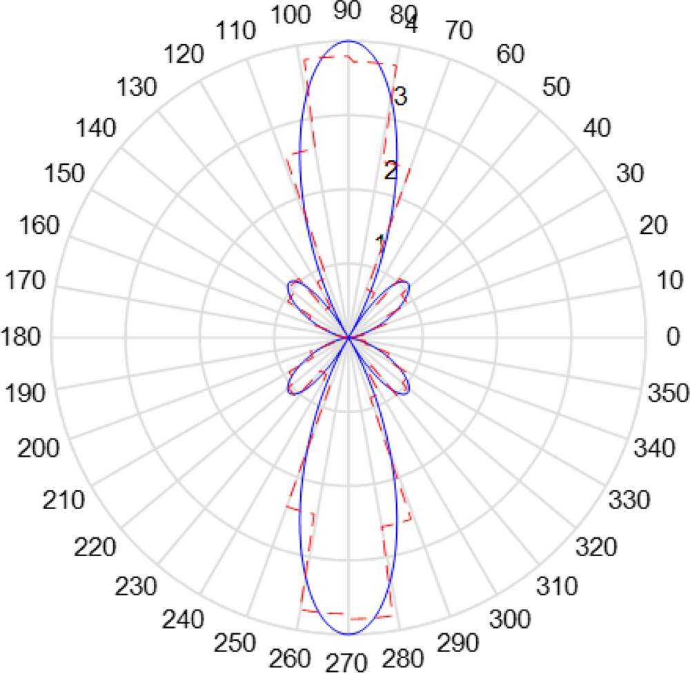
Figure 2: Piecewise model on antenna pattern.

With the piecewise model, the power constraint is given by (7)

$$\frac{4\pi r^2}{S}{\sum }_s{W}_s=P,$$

(7)

where $W_s$ is the power flow density. Therefore, the sum of $W_n$ representing the antenna radiation power flow density at the angle where the nth cluster is located is given by (8)

$${\sum }_n{W}_n\le \frac{P}{4\pi r^2}*S,$$

(8)

more precisely,

$${\sum }_n{W}_{s_n}=\frac{P}{4\pi r^2}*S*\gamma ,$$

(9)

where $\gamma$ is the ratio of the sum of the power in the angle of the channel clusters to the total power, which depends on the ability of the antenna to depress the beam at an uninterest angle.

In (1), the distance attenuation factor $\frac{1}{4\pi r^2}$ has been included in $h_n$ as the path loss factor, and P has been picked in the capacity expression of (4.a), so the power constraint of F is given by (10),

$${\sum }_n{\left|f_{t_m}(Ao{D}_n,Zo{D}_n)\right|}^2=S*\gamma \le S,$$

(10)

here, the beam convergence factor is defined as (11)

$$\mathrm{\rho }=S*\gamma ,$$

(11)

which represents the ability of the antenna to converge beams in the spatial clusters of interest, and is affected by actual antenna parameters. In the subsequent calculation, the beam convergence factor is given as known. The calculation results below show that the beam convergence factor does not change the shape of the pattern, but only affects the power distribution in Rss.

D. Problem solving

After the constraint shown in (10), (6) is rewritten by (12),

$\underset{(F,R_{ss})}{maximize}$	${\log }_2\det (I_M+{\displaystyle \frac{P}{{\sigma }^2}}{\tilde{H}}_{M\times N}*F_{N\times K}*R_{ss}$
$*F^H{}_{K\times N}*\tilde{H}^H{}_{N\times M}),$	(12.a)

subject to

$$Tr\left(R_{ss}\right)=1,$$

(12.b)

$${\sum }_n{\left|f_{t_m}(Ao{D}_n,Zo{D}_n)\right|}^2=S*\gamma ,\mathrm{for}\mathrm{m}=1,\mathrm{\dots },\mathrm{M},$$

(12.c)

Under the constraint in F, $F_{N\times K}*R_{ss}*F^H{}_{K\times N}$ is a symmetric positive definite matrix. Therefore, the optimal solution of F is the right singular matrix of ${\tilde{H}}_{M\times N}$ [25] and $R_{ss}$ can be obtained by the water-filling algorithm [25].

The singular value matrix is a unitary matrix, and any two columns of it are orthogonal. Therefore, the patterns of different transmitting antennas are orthogonal to each other in the clusters’ direction. Meanwhile, in order to ensure a higher signal-to-noise ratio at the receiver, the beam convergence factor should be greater, that means the smaller the gain in the angles except the spatial clusters’ direction, the better.

$${\tilde{H}}_{2\times 3}^{user1}=\left[\begin{array}{ccc}\hfill h_1^1\hfill & \hfill h_2^1\hfill & \hfill h_3^1\hfill \\ \hfill h_1^1{e}^{j\pi *\cos \left(Ao{A}_1^1\right)*\cos (Zo{A}_1^1)}\hfill & \hfill h_2^1{e}^{j\pi *\cos \left(Ao{A}_2^1\right)*\cos (Zo{A}_2^1)}\hfill & \hfill h_3^1{e}^{j\pi *\cos \left(Ao{A}_3^1\right)*\cos (Zo{A}_3^1)}\hfill \end{array}\right],$$

(13)

$${\tilde{H}}_{2\times 3}^{user2}=\left[\begin{array}{ccc}\hfill h_1^2\hfill & \hfill h_2^2\hfill & \hfill h_3^2\hfill \\ \hfill h_1^2{e}^{j\pi *\cos \left(Ao{A}_1^2\right)*\cos (Zo{A}_1^1)}\hfill & \hfill h_2^2{e}^{j\pi *\cos \left(Ao{A}_2^2\right)*\cos (Zo{A}_2^2)}\hfill & \hfill h_3^1{e}^{j\pi *\cos \left(Ao{A}_3^2\right)*\cos (Zo{A}_3^2)}\hfill \end{array}\right],$$

(14)

$F_{3\times 4}^{user1}$	(15)
$=\left[\begin{array}{cc}\hfill \begin{array}{cc}\hfill f_{t_1}(Ao{D}_1^1,Zo{D}_1^1)\hfill & \hfill f_{t_2}(Ao{D}_1^1,Zo{D}_1^1)e^{j\pi *\cos \left(Ao{D}_1^1\right)*\cos \left(Zo{D}_1^1\right)}\hfill \\ \hfill f_{t_1}(Ao{D}_2^1,Zo{D}_2^1)\hfill & \hfill f_{t_2}(Ao{D}_2^1,Zo{D}_2^1)e^{j\pi *\cos \left(Ao{D}_2^1\right)*\cos \left(Zo{D}_2^1\right)}\hfill \\ \hfill f_{t_1}(Ao{D}_3^1,Zo{D}_3^1)\hfill & \hfill f_{t_2}(Ao{D}_3^1,Zo{D}_3^1)e^{j\pi *\cos \left(Ao{D}_3^1\right)*\cos \left(Zo{D}_3^1\right)}\hfill \end{array}\hfill & \hfill \begin{array}{cc}\hfill f_{t_3}(Ao{D}_1^1,Zo{D}_1^1)e^{j2\pi *\cos \left(Ao{D}_1^1\right)*\cos \left(Zo{D}_1^1\right)}\hfill & \hfill f_{t_4}(Ao{D}_1^1,Zo{D}_1^1)e^{j3\pi *\cos \left(Ao{D}_1^1\right)*\cos \left(Zo{D}_1^1\right)}\hfill \\ \hfill f_{t_3}(Ao{D}_2^1,Zo{D}_2^1)e^{j2\pi *\cos \left(Ao{D}_2^1\right)*\cos \left(Zo{D}_2^1\right)}\hfill & \hfill f_{t_4}(Ao{D}_2^1,Zo{D}_2^1)e^{j3\pi *\cos \left(Ao{D}_2^1\right)*\cos \left(Zo{D}_2^1\right)}\hfill \\ \hfill f_{t_3}(Ao{D}_3^1,Zo{D}_3^1)e^{j2\pi *\cos \left(Ao{D}_3^1\right)*\cos \left(Zo{D}_3^1\right)}\hfill & \hfill f_{t_4}(Ao{D}_3^1,Zo{D}_3^1)e^{j3\pi *\cos \left(Ao{D}_3^1\right)*\cos \left(Zo{D}_3^1\right)}\hfill \end{array}\hfill \end{array}\right]$
$F_{3\times 4}^{user2}$	(16)
$=\left[\begin{array}{cc}\hfill \begin{array}{cc}\hfill f_{t_1}(Ao{D}_1^2,Zo{D}_1^2)\hfill & \hfill f_{t_2}(Ao{D}_1^2,Zo{D}_1^2)e^{j\pi *\cos \left(Ao{D}_1^2\right)*\cos \left(Zo{D}_1^2\right)}\hfill \\ \hfill f_{t_1}(Ao{D}_2^2,Zo{D}_2^2)\hfill & \hfill f_{t_2}(Ao{D}_2^2,Zo{D}_2^2)e^{j\pi *\cos \left(Ao{D}_2^2\right)*\cos \left(Zo{D}_2^2\right)}\hfill \\ \hfill f_{t_1}(Ao{D}_3^2,Zo{D}_3^2)\hfill & \hfill f_{t_2}(Ao{D}_3^2,Zo{D}_3^2)e^{j\pi *\cos \left(Ao{D}_3^2\right)*\cos \left(Zo{D}_3^2\right)}\hfill \end{array}\hfill & \hfill \begin{array}{cc}\hfill f_{t_3}(Ao{D}_1^2,Zo{D}_1^2)e^{j2\pi *\cos \left(Ao{D}_1^2\right)*\cos \left(Zo{D}_1^2\right)}\hfill & \hfill f_{t_4}(Ao{D}_1^2,Zo{D}_1^2)e^{j3\pi *\cos \left(Ao{D}_1^2\right)*\cos \left(Zo{D}_1^2\right)}\hfill \\ \hfill f_{t_3}(Ao{D}_2^2,Zo{D}_2^2)e^{j2\pi *\cos \left(Ao{D}_2^2\right)*\cos \left(Zo{D}_2^2\right)}\hfill & \hfill f_{t_4}(Ao{D}_2^2,Zo{D}_2^2)e^{j3\pi *\cos \left(Ao{D}_2^2\right)*\cos \left(Zo{D}_2^2\right)}\hfill \\ \hfill f_{t_3}(Ao{D}_3^2,Zo{D}_3^2)e^{j2\pi *\cos \left(Ao{D}_3^2\right)*\cos \left(Zo{D}_3^2\right)}\hfill & \hfill f_{t_4}(Ao{D}_3^2,Zo{D}_3^2)e^{j3\pi *\cos \left(Ao{D}_3^2\right)*\cos \left(Zo{D}_3^2\right)}\hfill \end{array}\hfill \end{array}\right]$
${\mathrm{F}}_{6\times 4}$	$=\left[\begin{array}{c}\hfill {\mathrm{F}}_{3\times 4}^{\mathrm{user1}}\hfill \\ \hfill {\mathrm{F}}_{3\times 4}^{\mathrm{user2}}\hfill \end{array}\right]$	(17)
$=\left[\begin{array}{c}\hfill \begin{array}{cc}\hfill \begin{array}{cc}\hfill {\mathrm{f}}_{{\mathrm{t}}_1}({\mathrm{AoD}}_1^1,{\mathrm{ZoD}}_1^1)\hfill & \hfill {\mathrm{f}}_{{\mathrm{t}}_2}({\mathrm{AoD}}_1^1,{\mathrm{ZoD}}_1^1){\mathrm{e}}^{\mathrm{j}\pi *\cos \left({\mathrm{AoD}}_1^1\right)*\cos \left({\mathrm{ZoD}}_1^1\right)}\hfill \\ \hfill {\mathrm{f}}_{{\mathrm{t}}_1}({\mathrm{AoD}}_2^1,{\mathrm{ZoD}}_2^1)\hfill & \hfill {\mathrm{f}}_{{\mathrm{t}}_2}({\mathrm{AoD}}_2^1,{\mathrm{ZoD}}_2^1){\mathrm{e}}^{\mathrm{j}\pi *\cos \left({\mathrm{AoD}}_2^1\right)*\cos \left({\mathrm{ZoD}}_2^1\right)}\hfill \\ \hfill {\mathrm{f}}_{{\mathrm{t}}_1}({\mathrm{AoD}}_3^1,{\mathrm{ZoD}}_3^1)\hfill & \hfill {\mathrm{f}}_{{\mathrm{t}}_2}({\mathrm{AoD}}_3^1,{\mathrm{ZoD}}_3^1){\mathrm{e}}^{\mathrm{j}\pi *\cos \left({\mathrm{AoD}}_3^1\right)*\cos \left({\mathrm{ZoD}}_3^1\right)}\hfill \end{array}\hfill & \hfill \begin{array}{cc}\hfill {\mathrm{f}}_{{\mathrm{t}}_3}({\mathrm{AoD}}_1^1,{\mathrm{ZoD}}_1^1){\mathrm{e}}^{\mathrm{j2}\pi *\cos \left({\mathrm{AoD}}_1^1\right)*\cos \left({\mathrm{ZoD}}_1^1\right)}\hfill & \hfill {\mathrm{f}}_{{\mathrm{t}}_4}({\mathrm{AoD}}_1^1,{\mathrm{ZoD}}_1^1){\mathrm{e}}^{\mathrm{j3}\pi *\cos \left({\mathrm{AoD}}_1^1\right)*\cos \left({\mathrm{ZoD}}_1^1\right)}\hfill \\ \hfill {\mathrm{f}}_{{\mathrm{t}}_3}({\mathrm{AoD}}_2^1,{\mathrm{ZoD}}_2^1){\mathrm{e}}^{\mathrm{j2}\pi *\cos \left({\mathrm{AoD}}_2^1\right)*\cos \left({\mathrm{ZoD}}_2^1\right)}\hfill & \hfill {\mathrm{f}}_{{\mathrm{t}}_4}({\mathrm{AoD}}_2^1,{\mathrm{ZoD}}_2^1){\mathrm{e}}^{\mathrm{j3}\pi *\cos \left({\mathrm{AoD}}_2^1\right)*\cos \left({\mathrm{ZoD}}_2^1\right)}\hfill \\ \hfill {\mathrm{f}}_{{\mathrm{t}}_3}({\mathrm{AoD}}_3^1,{\mathrm{ZoD}}_3^1){\mathrm{e}}^{\mathrm{j2}\pi *\cos \left({\mathrm{AoD}}_3^1\right)*\cos \left({\mathrm{ZoD}}_3^1\right)}\hfill & \hfill {\mathrm{f}}_{{\mathrm{t}}_4}({\mathrm{AoD}}_3^1,{\mathrm{ZoD}}_3^1){\mathrm{e}}^{\mathrm{j3}\pi *\cos \left({\mathrm{AoD}}_3^1\right)*\cos \left({\mathrm{ZoD}}_3^1\right)}\hfill \end{array}\hfill \end{array}\hfill \\ \hfill \begin{array}{cc}\hfill \begin{array}{cc}\hfill {\mathrm{f}}_{{\mathrm{t}}_1}({\mathrm{AoD}}_1^2,{\mathrm{ZoD}}_1^2)\hfill & \hfill {\mathrm{f}}_{{\mathrm{t}}_2}({\mathrm{AoD}}_1^2,{\mathrm{ZoD}}_1^2){\mathrm{e}}^{\mathrm{j}\pi *\cos \left({\mathrm{AoD}}_1^2\right)*\cos \left({\mathrm{ZoD}}_1^2\right)}\hfill \\ \hfill {\mathrm{f}}_{{\mathrm{t}}_1}({\mathrm{AoD}}_2^2,{\mathrm{ZoD}}_2^2)\hfill & \hfill {\mathrm{f}}_{{\mathrm{t}}_2}({\mathrm{AoD}}_2^2,{\mathrm{ZoD}}_2^2){\mathrm{e}}^{\mathrm{j}\pi *\cos \left({\mathrm{AoD}}_2^2\right)*\cos \left({\mathrm{ZoD}}_2^2\right)}\hfill \\ \hfill {\mathrm{f}}_{{\mathrm{t}}_1}({\mathrm{AoD}}_3^2,{\mathrm{ZoD}}_3^2)\hfill & \hfill {\mathrm{f}}_{{\mathrm{t}}_2}({\mathrm{AoD}}_3^2,{\mathrm{ZoD}}_3^2){\mathrm{e}}^{\mathrm{j}\pi *\cos \left({\mathrm{AoD}}_3^2\right)*\cos \left({\mathrm{ZoD}}_3^2\right)}\hfill \end{array}\hfill & \hfill \begin{array}{cc}\hfill {\mathrm{f}}_{{\mathrm{t}}_3}({\mathrm{AoD}}_1^2,{\mathrm{ZoD}}_1^2){\mathrm{e}}^{\mathrm{j2}\pi *\cos \left({\mathrm{AoD}}_1^2\right)*\cos \left({\mathrm{ZoD}}_1^2\right)}\hfill & \hfill {\mathrm{f}}_{{\mathrm{t}}_4}({\mathrm{AoD}}_1^2,{\mathrm{ZoD}}_1^2){\mathrm{e}}^{\mathrm{j3}\pi *\cos \left({\mathrm{AoD}}_1^2\right)*\cos \left({\mathrm{ZoD}}_1^2\right)}\hfill \\ \hfill {\mathrm{f}}_{{\mathrm{t}}_3}({\mathrm{AoD}}_2^2,{\mathrm{ZoD}}_2^2){\mathrm{e}}^{\mathrm{j2}\pi *\cos \left({\mathrm{AoD}}_2^2\right)*\cos \left({\mathrm{ZoD}}_2^2\right)}\hfill & \hfill {\mathrm{f}}_{{\mathrm{t}}_4}({\mathrm{AoD}}_2^2,{\mathrm{ZoD}}_2^2){\mathrm{e}}^{\mathrm{j3}\pi *\cos \left({\mathrm{AoD}}_2^2\right)*\cos \left({\mathrm{ZoD}}_2^2\right)}\hfill \\ \hfill {\mathrm{f}}_{{\mathrm{t}}_3}({\mathrm{AoD}}_3^2,{\mathrm{ZoD}}_3^2){\mathrm{e}}^{\mathrm{j2}\pi *\cos \left({\mathrm{AoD}}_3^2\right)*\cos \left({\mathrm{ZoD}}_3^2\right)}\hfill & \hfill {\mathrm{f}}_{{\mathrm{t}}_4}({\mathrm{AoD}}_3^2,{\mathrm{ZoD}}_3^2){\mathrm{e}}^{\mathrm{j3}\pi *\cos \left({\mathrm{AoD}}_3^2\right)*\cos \left({\mathrm{ZoD}}_3^2\right)}\hfill \end{array}\hfill \end{array}\hfill \end{array}\right]$
${\tilde{\mathrm{H}}}_{2\times 6}^1=\left[\begin{array}{cc}\hfill {\tilde{\mathrm{H}}}_{2\times 3}^{\mathrm{user1}}\hfill & \hfill 0\hfill \end{array}\right]=\left[\begin{array}{cc}\hfill \begin{array}{ccc}\hfill {\mathrm{h}}_1^1\hfill & \hfill {\mathrm{h}}_2^1\hfill & \hfill {\mathrm{h}}_3^1\hfill \\ \hfill {\mathrm{h}}_1^1{\mathrm{e}}^{\mathrm{j}\pi *\cos \left({\mathrm{AoA}}_1^1\right)*\cos ({\mathrm{ZoA}}_1^1)}\hfill & \hfill {\mathrm{h}}_2^1{\mathrm{e}}^{\mathrm{j}\pi *\cos \left({\mathrm{AoA}}_2^1\right)*\cos ({\mathrm{ZoA}}_2^1)}\hfill & \hfill {\mathrm{h}}_3^1{\mathrm{e}}^{\mathrm{j}\pi *\cos \left({\mathrm{AoA}}_3^1\right)*\cos ({\mathrm{ZoA}}_3^1)}\hfill \end{array}\hfill & \hfill \begin{array}{ccc}\hfill 0\hfill & \hfill 0\hfill & \hfill 0\hfill \\ \hfill 0\hfill & \hfill 0\hfill & \hfill 0\hfill \end{array}\hfill \end{array}\right],$	(18)
${\tilde{\mathrm{H}}}_{2\times 6}^2=\left[\begin{array}{cc}\hfill 0\hfill & \hfill {\tilde{\mathrm{H}}}_{2\times 3}^{\mathrm{user2}}\hfill \end{array}\right]=\left[\begin{array}{cc}\hfill \begin{array}{ccc}\hfill 0\hfill & \hfill 0\hfill & \hfill 0\hfill \\ \hfill 0\hfill & \hfill 0\hfill & \hfill 0\hfill \end{array}\hfill & \hfill \begin{array}{ccc}\hfill {\mathrm{h}}_1^2\hfill & \hfill {\mathrm{h}}_2^2\hfill & \hfill {\mathrm{h}}_3^2\hfill \\ \hfill {\mathrm{h}}_1^2{\mathrm{e}}^{\mathrm{j}\pi *\cos \left({\mathrm{AoA}}_1^2\right)*\cos ({\mathrm{ZoA}}_1^1)}\hfill & \hfill {\mathrm{h}}_2^2{\mathrm{e}}^{\mathrm{j}\pi *\cos \left({\mathrm{AoA}}_2^2\right)*\cos ({\mathrm{ZoA}}_2^2)}\hfill & \hfill {\mathrm{h}}_3^1{\mathrm{e}}^{\mathrm{j}\pi *\cos \left({\mathrm{AoA}}_3^2\right)*\cos ({\mathrm{ZoA}}_3^2)}\hfill \end{array}\hfill \end{array}\right],$	(19)
$\begin{array}{cc}\hfill {\mathrm{H}}_{4\times 4}=& \left[\begin{array}{c}\hfill {\tilde{\mathrm{H}}}_{2\times 6}^1\hfill \\ \hfill {\tilde{\mathrm{H}}}_{2\times 6}^2\hfill \end{array}\right]*\left[\begin{array}{c}\hfill {\mathrm{F}}_{3\times 4}^{\mathrm{user1}}\hfill \\ \hfill {\mathrm{F}}_{3\times 4}^{\mathrm{user2}}\hfill \end{array}\right]={\tilde{\mathrm{H}}}_{4\times 6}*{\mathrm{F}}_{6\times 4}\hfill \\ \hfill =& \left[\begin{array}{cccccc}\hfill {\mathrm{h}}_1^1\hfill & \hfill {\mathrm{h}}_2^1\hfill & \hfill {\mathrm{h}}_3^1\hfill & \hfill 0\hfill & \hfill 0\hfill & \hfill 0\hfill \\ \hfill {\mathrm{h}}_1^1{\mathrm{e}}^{\mathrm{j}\pi *\cos \left({\mathrm{AoA}}_1^1\right)*\cos \left({\mathrm{ZoA}}_1^1\right)}\hfill & \hfill {\mathrm{h}}_2^1{\mathrm{e}}^{\mathrm{j}\pi *\cos \left({\mathrm{AoA}}_2^1\right)*\cos \left({\mathrm{ZoA}}_2^1\right)}\hfill & \hfill {\mathrm{h}}_3^1{\mathrm{e}}^{\mathrm{j}\pi *\cos \left({\mathrm{AoA}}_3^1\right)*\cos \left({\mathrm{ZoA}}_3^1\right)}\hfill & \hfill 0\hfill & \hfill 0\hfill & \hfill 0\hfill \\ \hfill 0\hfill & \hfill 0\hfill & \hfill 0\hfill & \hfill {\mathrm{h}}_3^1\hfill & \hfill {\mathrm{h}}_2^2\hfill & \hfill {\mathrm{h}}_2^2\hfill \\ \hfill 0\hfill & \hfill 0\hfill & \hfill 0\hfill & \hfill {\mathrm{h}}_3^1{\mathrm{e}}^{\mathrm{j}\pi *\cos \left({\mathrm{AoA}}_3^1\right)*\cos \left({\mathrm{ZoA}}_3^1\right)}\hfill & \hfill {\mathrm{h}}_2^2{\mathrm{e}}^{\mathrm{j}\pi *\cos \left({\mathrm{AoA}}_2^2\right)*\cos \left({\mathrm{ZoA}}_2^2\right)}\hfill & \hfill {\mathrm{h}}_2^2{\mathrm{e}}^{\mathrm{j}\pi *\cos \left({\mathrm{AoA}}_2^2\right)*\cos \left({\mathrm{ZoA}}_2^2\right)}\hfill \end{array}\right]\hfill \\ & *\left[\begin{array}{cccc}\hfill {\mathrm{f}}_{{\mathrm{t}}_1}({\mathrm{AoD}}_1^1,{\mathrm{ZoD}}_1^1)\hfill & \hfill {\mathrm{f}}_{{\mathrm{t}}_2}({\mathrm{AoD}}_1^1,{\mathrm{ZoD}}_1^1){\mathrm{e}}^{\mathrm{j}\pi *\cos \left({\mathrm{AoD}}_1^1\right)*\cos \left({\mathrm{ZoD}}_1^1\right)}\hfill & \hfill {\mathrm{f}}_{{\mathrm{t}}_3}({\mathrm{AoD}}_1^1,{\mathrm{ZoD}}_1^1){\mathrm{e}}^{\mathrm{j2}\pi *\cos \left({\mathrm{AoD}}_1^1\right)*\cos \left({\mathrm{ZoD}}_1^1\right)}\hfill & \hfill {\mathrm{f}}_{{\mathrm{t}}_4}({\mathrm{AoD}}_1^1,{\mathrm{ZoD}}_1^1){\mathrm{e}}^{\mathrm{j3}\pi *\cos \left({\mathrm{AoD}}_1^1\right)*\cos \left({\mathrm{ZoD}}_1^1\right)}\hfill \\ \hfill {\mathrm{f}}_{{\mathrm{t}}_1}({\mathrm{AoD}}_2^1,{\mathrm{ZoD}}_2^1)\hfill & \hfill {\mathrm{f}}_{{\mathrm{t}}_2}({\mathrm{AoD}}_2^1,{\mathrm{ZoD}}_2^1){\mathrm{e}}^{\mathrm{j}\pi *\cos \left({\mathrm{AoD}}_2^1\right)*\cos \left({\mathrm{ZoD}}_2^1\right)}\hfill & \hfill {\mathrm{f}}_{{\mathrm{t}}_3}({\mathrm{AoD}}_2^1,{\mathrm{ZoD}}_2^1){\mathrm{e}}^{\mathrm{j2}\pi *\cos \left({\mathrm{AoD}}_2^1\right)*\cos \left({\mathrm{ZoD}}_2^1\right)}\hfill & \hfill {\mathrm{f}}_{{\mathrm{t}}_4}({\mathrm{AoD}}_2^1,{\mathrm{ZoD}}_2^1){\mathrm{e}}^{\mathrm{j3}\pi *\cos \left({\mathrm{AoD}}_2^1\right)*\cos \left({\mathrm{ZoD}}_2^1\right)}\hfill \\ \hfill {\mathrm{f}}_{{\mathrm{t}}_1}({\mathrm{AoD}}_3^1,{\mathrm{ZoD}}_3^1)\hfill & \hfill {\mathrm{f}}_{{\mathrm{t}}_2}({\mathrm{AoD}}_3^1,{\mathrm{ZoD}}_3^1){\mathrm{e}}^{\mathrm{j}\pi *\cos \left({\mathrm{AoD}}_3^1\right)*\cos \left({\mathrm{ZoD}}_3^1\right)}\hfill & \hfill {\mathrm{f}}_{{\mathrm{t}}_3}({\mathrm{AoD}}_3^1,{\mathrm{ZoD}}_3^1){\mathrm{e}}^{\mathrm{j2}\pi *\cos \left({\mathrm{AoD}}_3^1\right)*\cos \left({\mathrm{ZoD}}_3^1\right)}\hfill & \hfill {\mathrm{f}}_{{\mathrm{t}}_4}({\mathrm{AoD}}_3^1,{\mathrm{ZoD}}_3^1){\mathrm{e}}^{\mathrm{j3}\pi *\cos \left({\mathrm{AoD}}_3^1\right)*\cos \left({\mathrm{ZoD}}_3^1\right)}\hfill \\ \hfill {\mathrm{f}}_{{\mathrm{t}}_1}({\mathrm{AoD}}_1^2,{\mathrm{ZoD}}_1^2)\hfill & \hfill {\mathrm{f}}_{{\mathrm{t}}_2}({\mathrm{AoD}}_1^2,{\mathrm{ZoD}}_1^2){\mathrm{e}}^{\mathrm{j}\pi *\cos \left({\mathrm{AoD}}_1^2\right)*\cos \left({\mathrm{ZoD}}_1^2\right)}\hfill & \hfill {\mathrm{f}}_{{\mathrm{t}}_3}({\mathrm{AoD}}_1^2,{\mathrm{ZoD}}_1^2){\mathrm{e}}^{\mathrm{j2}\pi *\cos \left({\mathrm{AoD}}_1^2\right)*\cos \left({\mathrm{ZoD}}_1^2\right)}\hfill & \hfill {\mathrm{f}}_{{\mathrm{t}}_4}({\mathrm{AoD}}_1^2,{\mathrm{ZoD}}_1^2){\mathrm{e}}^{\mathrm{j3}\pi *\cos \left({\mathrm{AoD}}_1^2\right)*\cos \left({\mathrm{ZoD}}_1^2\right)}\hfill \\ \hfill {\mathrm{f}}_{{\mathrm{t}}_1}({\mathrm{AoD}}_2^2,{\mathrm{ZoD}}_2^2)\hfill & \hfill {\mathrm{f}}_{{\mathrm{t}}_2}({\mathrm{AoD}}_2^2,{\mathrm{ZoD}}_2^2){\mathrm{e}}^{\mathrm{j}\pi *\cos \left({\mathrm{AoD}}_2^2\right)*\cos \left({\mathrm{ZoD}}_2^2\right)}\hfill & \hfill {\mathrm{f}}_{{\mathrm{t}}_3}({\mathrm{AoD}}_2^2,{\mathrm{ZoD}}_2^2){\mathrm{e}}^{\mathrm{j2}\pi *\cos \left({\mathrm{AoD}}_2^2\right)*\cos \left({\mathrm{ZoD}}_2^2\right)}\hfill & \hfill {\mathrm{f}}_{{\mathrm{t}}_4}({\mathrm{AoD}}_2^2,{\mathrm{ZoD}}_2^2){\mathrm{e}}^{\mathrm{j3}\pi *\cos \left({\mathrm{AoD}}_2^2\right)*\cos \left({\mathrm{ZoD}}_2^2\right)}\hfill \\ \hfill {\mathrm{f}}_{{\mathrm{t}}_1}({\mathrm{AoD}}_3^2,{\mathrm{ZoD}}_3^2)\hfill & \hfill {\mathrm{f}}_{{\mathrm{t}}_2}({\mathrm{AoD}}_3^2,{\mathrm{ZoD}}_3^2){\mathrm{e}}^{\mathrm{j}\pi *\cos \left({\mathrm{AoD}}_3^2\right)*\cos \left({\mathrm{ZoD}}_3^2\right)}\hfill & \hfill {\mathrm{f}}_{{\mathrm{t}}_3}({\mathrm{AoD}}_3^2,{\mathrm{ZoD}}_3^2){\mathrm{e}}^{\mathrm{j2}\pi *\cos \left({\mathrm{AoD}}_3^2\right)*\cos \left({\mathrm{ZoD}}_3^2\right)}\hfill & \hfill {\mathrm{f}}_{{\mathrm{t}}_4}({\mathrm{AoD}}_3^2,{\mathrm{ZoD}}_3^2){\mathrm{e}}^{\mathrm{j3}\pi *\cos \left({\mathrm{AoD}}_3^2\right)*\cos \left({\mathrm{ZoD}}_3^2\right)}\hfill \end{array}\right].\hfill \end{array}$	(20)

III. OPTIMAL ANTENNA DESIGN OF MIMO-MU

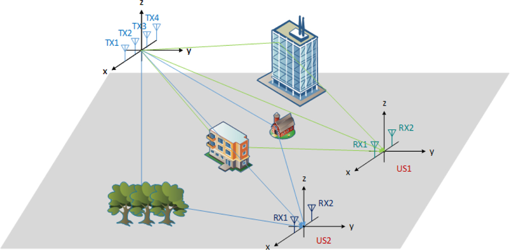
Figure 3: Channel with two users.

In the MIMO-MU channel, shown in Fig. 3, the wireless propagation environment matrix for user 1 and user 2 are given by (13) and (14). F matrix for user 1 and user 2 are given by (15) and (16).

where $h_n^u$ is the gain of nth cluster for the uth user. $Ao{A}_n^u$, $Zo{A}_n^u$, $Ao{D}_n^u$ and $Zo{D}_n^u$ are the angles of the nth cluster for the uth user. Rewrite F as (17), rewrite ${\tilde{H}}_{2\times 3}^{user1}$ as ${\tilde{H}}_{2\times 6}^1$ shown as (18), rewrite ${\tilde{H}}_{2\times 3}^{user2}$ as ${\tilde{H}}_{2\times 6}^2$ shown as (19). The channel coefficients matrix between 4 receiving antennas and 4 transmitting antennas for MIMO-MU is givenby (20).

Therefore, the capacity for MIMO-MU is given by (21),

$$\mathrm{C}={\log }_2\det \left(I_4+\frac{P}{{\sigma }^2}{\tilde{H}}_{4\times 6}*F_{6\times 4}*R_{ss}*F_{4\times 6}^H*\tilde{H}^H{}_{6\times 4}\right).$$

(21)

Using the same solution in subsection D, the optimal patterns of F is the right singular matrix of ${\tilde{H}}_{4\times 6}$, and $R_{ss}$ can be obtained by the water-filling algorithm.

Because ${\tilde{H}}_{4\times 6}$ is block matrix, the optimal F is block matrix too, which is given by (22),

$$F_{6\times 4}=\left[\begin{array}{cc}\hfill \begin{array}{c}\hfill V_{3\times 2}^1\hfill \\ \hfill 0\hfill \end{array}\hfill & \hfill \begin{array}{c}\hfill 0\hfill \\ \hfill V_{3\times 2}^2\hfill \end{array}\hfill \end{array}\right],$$	(22.a)
$${\tilde{H}}_{2\times 3}^{user1}=U_{2\times 3}^1{S}_{3\times 3}^1{V}_{3\times 3}^1,$$	(22.b)
$${\tilde{H}}_{2\times 3}^{user2}=U_{2\times 3}^2{S}_{3\times 3}^2{V}_{3\times 3}^2,$$	(22.c)

where $V_{3\times 2}^1$ and $V_{3\times 2}^2$ are the two columns of $V_{3\times 3}^1$ and $V_{3\times 3}^2$ , which is the right singular matrix of ${\tilde{H}}_{2\times 3}^{user1}$ and ${\tilde{H}}_{2\times 3}^{user2}$. There are only two singular values for ${\tilde{H}}_{2\times 3}^{user1}$ and ${\tilde{H}}_{2\times 3}^{user2}$, so the third column of $V_{3\times 3}^1$ and $V_{3\times 3}^2$ are both zero vector.

The results in (22) show that the four antennas at the transmitter are divided into two groups. The first two antennas transmit beams to the spatial clusters of user 1, and the last two antennas transmit beams to the spatial clusters of user 2. The spatial decoupling between the two users is realized by the directivity of the transmission antennas.

On the spatial clusters of user 2, the beam gain of the first two transmit antennas should preferably be 0, otherwise it will cause interference to user 2; Similarly, on the spatial clusters of user 1, the beam gain of the last two antennas should preferably be 0, otherwise it will cause interference to user 1.

The above solution is only one of the most direct results of the optimal pattern. F can also be the vector space of the right singular vector of the wireless propagation environment channel matrix $\tilde{H}$. But it needs to cooperate with the digital baseband precoding to realize the decoupling of the data flow to the two users.

That is, the optimal F matrix should meet the following conditions:

1. Full rank

2. All singular values are equal

The above conditions can ensure that the loss of the condition number and the rank loss of the channel matrix H will not occur due to the rank loss of F or the bad condition number of F.

IV. SIMULATION

A. Simulation for MIMO-SU

In the QurdiGa channel model, the BERLIN_Uma_NLOS scenario is used to generate a wireless channel with 15 clusters, as shown in Fig. 4. The number of Tx antennas and Rx antennas are both 2. The total power is set to $10W$. The noise power is set to ${10}^{-12}mW$ which is close to the noise power of the phone 117dBm. According to the calculation in subsection D, the optimal pattern F is shown in Fig. 5. Corresponding to different beam convergence factors, the power distribution and capacity are shown inTable 1.

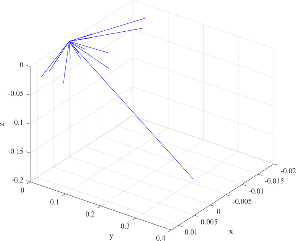
Figure 4: Clusters for MIMO-SU channel.

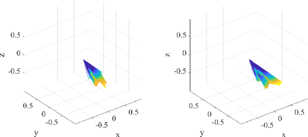
Figure 5: Optimal patterns for Tx1 (left) and Tx2(right).

Table 1: Power distribution and capacity

Beam Convergence Factor	PowerDistribution(W)	Capacity (bits/s/Hz)
$\mathrm{\rho }=1$	6.3411, 3.6589	6.7926
$\mathrm{\rho }=2$	5.6720, 4.3280	8.4427
$\mathrm{\rho }=3$	5.4468, 4.5532	9.4877
$\mathrm{\rho }=100$	5.0134, 4.9866	19.3404

Simulation results show that the patterns of different transmitting antennas are orthogonal to each other in the clusters’ direction; The increase of beam convergence factor will increase the gain of the transmitting antenna pattern in the direction of each transmitting cluster in equal proportion, but will not change the shape of the pattern; At the same time, the increase of beam convergence factor will make the transmission power distribution of each transmitting antenna closer. When the beam convergence factor is large, the capacity will be greatly improved, and the power distribution between antennas is close to average.

B. Simulation for MIMO-MU

In the MIMO-MU simulation, there is one sender with 8 antennas and three users with 2 antennaseach.

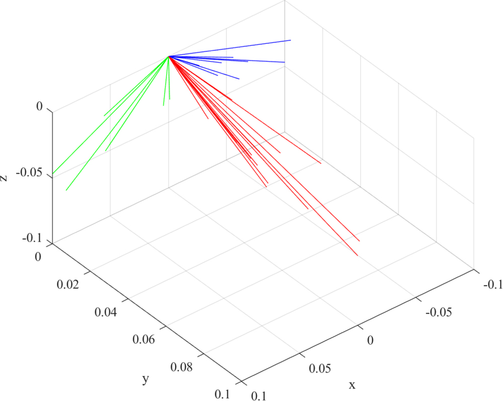
Figure 6: Clusters for MIMO-MU channel.

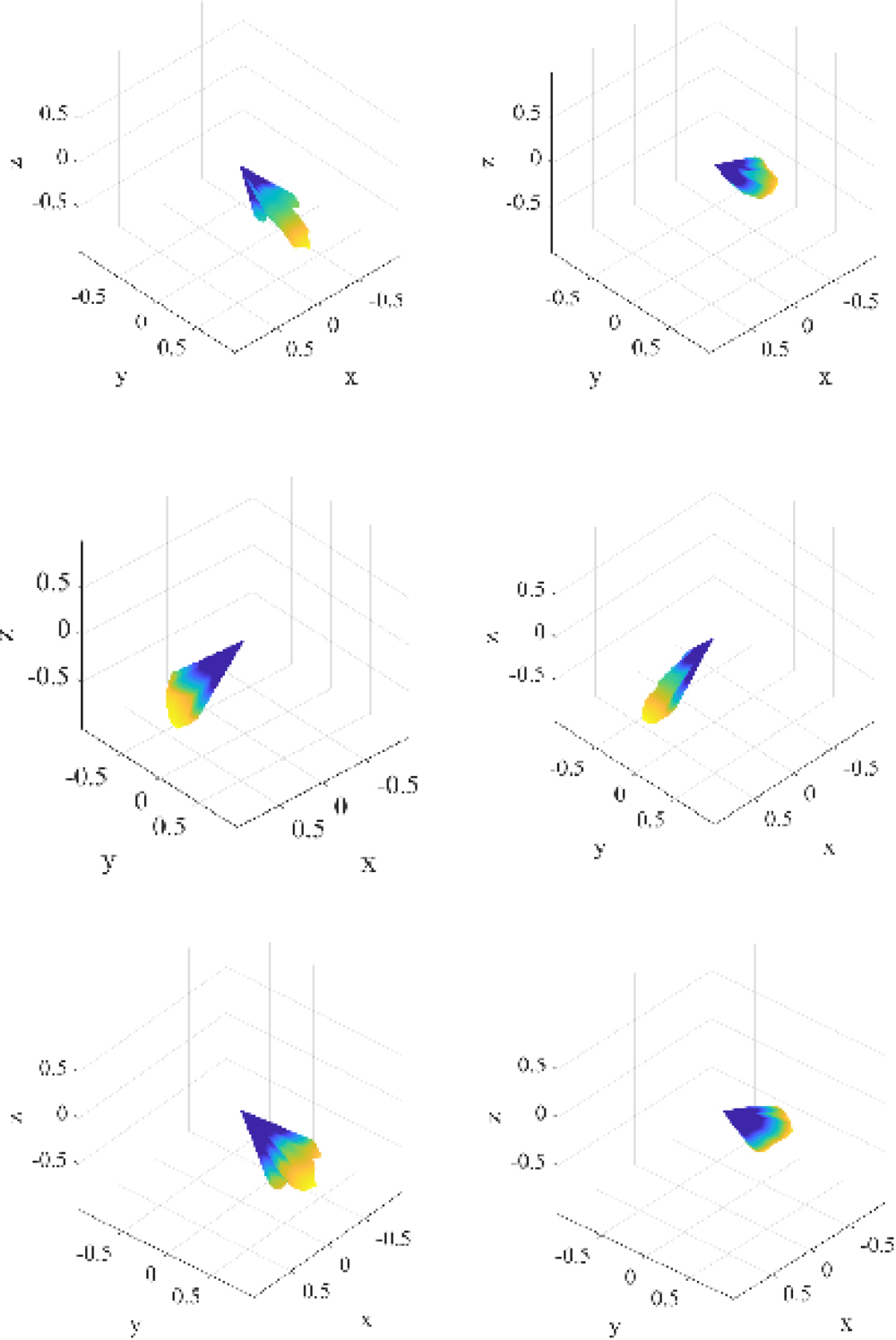
Figure 7: Optimal patterns for 6 Tx antennas.

Table 2: Power distribution and capacity in MIMO-MU

BeamConvergence Factor	Power Distribution(W)	Capacity(bits/s/Hz)
$\mathrm{\rho }=1$	1.9584, 1.8851,1.8406, 1.7178,1.6374, 0.9608,0.0000, 0.0000.	18.0202
$\mathrm{\rho }=2$	1.8127, 1.7761,1.7538, 1.6924,1.6522, 1.3128,0.0000, 0.0000.	23.2046
$\mathrm{\rho }=3$	1.7642, 1.7398,1.7250, 1.6837,1.6568, 1.4306,0.0000, 0.0000.	26.4202
$\mathrm{\rho }=100$	1.6734, 1.6729,1.6709, 1.6690,1.6641, 1.6498,0.0000, 0.0000.	50.2034

The MIMO-MU channel with 3 users is shown in Fig. 6. There are 15 clusters for each user. The right, middle and left parts of lines represent the propagation clusters pointing to user 1, user 2, and user 3. The lines’ direction in the figure represents the angle of the cluster, the length represents the cluster’s gain.

The optimal patterns for the first 6 Tx antennas are shown in Fig. 7. The power distribution is shown in Table 2.

The simulation results show that the first six antennas are exactly divided into three groups, each serving one user, and the last two antennas are not used, which is consistent with the analysis in Section III.

V. CONCLUSION

For the instantaneous MIMO channel based on the spatial cluster model, the product form of the channel coefficient matrix from the environment cluster matrix and transmit antenna pattern matrix has been given. Through piecewise modeling for the transmitting antenna pattern and power constraints, the optimization problem of maximizing the capacity has been solved by using singular value decomposition and the water-filling algorithm. The closed-form of the optimal antenna pattern has been achieved. The simulation results show the solution in this paper is effective.

REFERENCES

[1] C. Wang, F. Haider, X. Gao, X. You, Y. Yang, and D. Yuan, “Cellular architecture and key technologies for 5G wireless communication networks,” IEEE Comun. Mag., vol. 52, no. 2, pp. 122-130, Feb. 2014.

[2] Z. Pi and F. Khan, “An introduction to millimeter-wave mobile broadband systems,” IEEE Commun. Mag., vol. 49, no. 6, pp. 101-107, Jun. 2011.

[3] Z. Zhang, Y. Xiao, Z. Ma, M. Xiao, Z. Ding, X. Lei, G. K. Karaginanidis, and P. Fan, “6G wireless networks: vision, requirements, architecture, and key technologies,” IEEE Veh. Technol. Mag., vol. 14, no. 3, pp. 28-41, Sep. 2019.

[4] H. Pei, X. Chen, X. Huang, X. Liu, X. Zhang, and Y. Huang, “Key issues and algorithms of multiple-input-multiple-output over-the-air testing in the multi-probe anechoic chamber setup,” Sci. China Inf. Sci, vol. 65, no. 3, pp. 47-73, Mar. 2022.

[5] W. Hong, K.-H. Baek, Y. Lee, Y. Kim, and S.-T. Ko, “Study and prototyping of practically large-scale mmWave antenna systems for 5G cellular devices,” IEEE Commun. Mag., vol. 52, no. 9, pp. 63-69, Sep. 2014.

[6] B. T. Quist and M. A. Jensen, “Optimal antenna pattern design for MIMO systems,” IEEE Antennas and Propagation Society International Symposium, Honolulu, HI, USA, pp. 1905-1908, 2007.

[7] D. Evans and M. A. Jensen, “Near-optimal radiation characteristics for diversity antenna design,” IEEE International Workshop on Antenna Technology, Santa Monica, CA, USA, pp. 1-4, 2009.

[8] D. N. Evans and M. A. Jensen, “Near-optimal radiation patterns for antenna diversity,” IEEE Trans. Antennas Propag., vol. 58, no. 11, pp. 3765-3769, Nov. 2010.

[9] Y. Wang, X. Chen, H. Pei, W. Sha, H. Yi, and A. A. Kishk, “MIMO performance enhancement of MIMO arrays using PCS-based near-field optimization technique,” Sci. China Inf. Sci., in press, doi: 10.1007/s11432-022-3595-y.

[10] S. Song, Y. Da, B. Qian, X. Huang, X. Chen, Y. Li, and A. A. Kishk, “Dielectric resonator magnetoelectric dipole arrays with low cross polarization, backward radiation, and mutual coupling for MIMO base station applications,” China Commun., in press

[11] C. Feng, W. Shen, J. An, and L. Hanzo, “Joint hybrid and passive RIS-assisted beamforming for mmWave MIMO systems relying on dynamically configured subarrays,” IEEE IoT Journal, vol. 9, no. 15, pp. 13913-13926, Aug. 2022.

[12] Q. Zhu, R. Liu, Y. Liu, M. Li, and Q. Liu, “Joint design of hybrid and reflection beamforming for RIS-aided mmWave MIMO communications,” IEEE Globecom Workshops (GC Wkshps), Madrid, Spain, pp. 1-6, 2021.

[13] R. Deng, B. Di, H. Zhang, Y. Tan, and L. Song, “Reconfigurable holographic surface-enabled multi-user wireless communications: Amplitude-controlled holographic beamforming,” IEEE Trans. Wireless Commun., vol. 21, no. 8, pp. 6003-6017, Aug. 2022.

[14] R. Deng, B. Di, H. Zhang, and L. Song, “HDMA: holographic-pattern division multiple access,” IEEE J. Sel. Areas Commun., vol. 40, no. 4, pp. 1317-1332, Apr. 2022.

[15] C.-H. Hsu, “Optimizing uplink beam pattern of smart antenna by phase-amplitude disturbance in a linear array,” IEEE Antennas and Propagation Society Symposium, 2004, Monterey, CA, USA, vol. 3, pp. 2827-2830, 2004.

[16] S. Ma, H. Li, A. Cao, J. Tan, and J. Zhou, “Pattern synthesis of the distributed array based on the hybrid algorithm of particle swarm optimization and convex optimization,” 11th International Conference on Natural Computation (ICNC), Zhangjiajie, pp. 1230-1234, 2015.

[17] E. R. Schlosser, S. M. Tolfo, and M. V. T. Heckler, “Particle swarm optimization for antenna arrays synthesis,” SBMO/IEEE MTT-S International Microwave and Optoelectronics Conference (IMOC), Porto de Galinhas, Brazil, pp. 1-6,2015.

[18] A. Smida, R. Ghayoula, H. Trabelsi, and A. Gharsallah, “Adaptive radiation pattern optimization for antenna arrays by phase using a Taguchi Optimization method,” 11th Mediterranean Microwave Symposium (MMS), Yasmine Hammamet, Tunisia, pp. 138-141, 2011.

[19] A. Smida, R. Ghayoula, and A. Gharsallah, “Beamforming multibeam antenna array using Taguchi Optimization method,” 2nd World Symposium on Web Applications and Networking (WSWAN), Sousse, Tunisia, pp. 1-4, 2015.

[20] W. Shi, X. Liu, and Y. Li, “ULA fitting for MIMO radar,” IEEE Commun. Lett., vol. 26, no. 9, pp. 2190-2194, Sep. 2020.

[21] S. Luo, Y. Li, T. Jiang, and B. Li, “FSS and meta-material based low mutual coupling MIMO antenna array,” IEEE International Symposium on Antennas and Propagation and USNC-URSI Radio Science Meeting, Atlanta, GA, pp. 725-726, 2019.

[22] 3GPP. TR 38.901 V16.1.0, “5G; Study on channel model for frequencies from 0.5 to 100 GHz,” Nov. 2020.

[23] X. Chen, M. Zhao, H. Huang, Y. Wang, S. Zhu, C. Zhang, J. Yi, and A. A. Kishk, “Simultaneous decoupling and decorrelation scheme of MIMO arrays,” IEEE Trans. Veh. Technol., vol. 71, no. 2, pp. 2164-2169, Feb. 2022.

[24] Y. Wang, X. Chen, X. Liu, J. Yi, J. Chen, A. Zhang, and A. A. Kishk, “Improvement of diversity and capacity of MIMO system using scatterer array,” IEEE Trans. Antennas Propag., vol. 70, no. 1, pp. 789-794, Jan. 2022.

[25] J. R. Hampton, Introduction to MIMO Comunications, Cambridge University Press, Cambridge, UK, 2013.

BIOGRAPHIES

Cuicui Zhang received her B.S. and M.S. degrees in Information and Communications Engineering from Xi’an Jiaotong University, Xi’an, China, in 2010 and 2013. She is currently pursuing a Ph.D. degree in Electronics Science and Technology from Xi’an Jiaotong University, Xi’an, China. Her research interest is antenna design for 5G/6G MIMO systems.

Shuo Wang received his B.S. degree in Information Engineering from Xi’an Jiaotong University, Xi’an, China, in 2020. He is currently studying for an M.S. degree at the School of Information and Communications Engineering from Xi’an Jiaotong University, Xi’an, China. His research interest is communication algorithms related to reconfigurable antennas for 5G MIMOsystems.

Ming Zhang received his B.S. and M.S. degrees in Information and Communications Engineering, and his Ph.D. degree in Electronic Science and Technology, all from Xi’an Jiaotong University, Xi’an, China, in 2008, 2011, and 2017, respectively. From 2011 to 2014, he was with Huawei Technologies Co., Ltd., Xi’an, China. He is currently an associate professor at Xi’an Jiaotong University. His research interests include array signal processing and numerical optimization.

Xiaobo Liu (Member, IEEE) was born in Baoji, China, in 1992. He received his B.Eng. degree in Information Engineering and his Ph.D. degree in Electronic Science and Technology from Xi’an Jiaotong University, Xi’an, China, in 2014 and 2018, respectively. Since 2019, he has been a Research Associate at Xi’an Jiaotong University. He has authored or coauthored more than 20 articles in international and domestic journals and conferences. His research interests include electromagnetic fields and microwave theory, computational electromagnetics, metasurface, antenna design, and microwave circuits.

Anxue Zhang received his B.S. degree in Electrical Engineering from Henan Normal University, Henan, China, in 1996, and M.S. and Ph.D. degrees in Electrical Engineering from Xi’an Jiaotong University, Xi’an, China, in 1999 and 2003, respectively. He is currently a professor and director of the Institute of Electromagnetics and Information Technology of Xi’an Jiaotong University. He is also a member of the Academic Committee of the Key Laboratory of Ultra-High Speed Circuit Design and Electromagnetic Compatibility at the Ministry of Education. His research areas include antenna and electromagnetic wave propagation, RF and microwave circuit design, and metamaterials. He has coauthored one book, and more than 300 journal papers on these topics.

ACES JOURNAL, Vol. 37, No. 12, 1192–1199
doi: 10.13052/2022.ACES.J.371202
© 2022 River Publishers