Failure Mechanism Analysis of the Stochastic Galerkin Method in EMC Simulation Considering Geometric Randomness

Jinjun Bai, Bing Hu, and Yixuan Wan

College of Marine Electrical Engineering
Dalian Maritime University, Dalian, 116026, China
baijinjun@dlmu.edu.cn, hb1120221308@dlmu.edu.cn, wanyixuan@dlmu.edu.cn

Submitted On: December 17, 2023; Accepted On: September 22, 2023

ABSTRACT

By virtue of its high calculational accuracy and efficiency, the stochastic Galerkin method (SGM) has been successfully applied many times in electromagnetic compatibility (EMC) simulation in recent years. This paper proposes a calculating example taking geometric uncertainty factors into consideration. As is proved in the paper, there is a relatively large error when using the SGM to solve the example mentioned above. According to failure mechanism, the fundamental reason of the failure of the simulation lies in the additional error caused by using numerical integration to solve the inner product formula. Meanwhile, it is proved that no additional errors are introduced when using the stochastic collocation method (SCM), so the SCM is better than the SGM in stability. In the end, the paper revised the general selective strategy for uncertainty analysis methods, thus providing theoretical basis for their universal application in EMC field.

Index Terms: electromagnetic compatibility, failure mechanism analysis, stochastic collocation method, stochastic Galerkin method, uncertainty simulation method.

I. INTRODUCTION

Nowadays, uncertainty simulation methods are widely used in the field of electromagnetic compatibility (EMC) to accurately describe random factors in the actual engineering environment.

The Monte Carlo method (MCM) is the first uncertainty simulation method introduced into the EMC field, but its low computational efficiency renders it uncompetitive [1, 2]. At the same time, some efficient uncertainty simulation methods have also been proposed, such as the perturbation method [3, 4], the moment method [5, 6] and the stochastic reduced order models [7]. However, the calculation accuracy of these methods is not ideal. When the uncertainty of the EMC simulation input is large, the accuracy of the perturbation method will be severely reduced [4]. When the nonlinearity between the input and output of the EMC simulation is large, the moment method will fail [6]. For the stochastic reduced order models, the lack of effective method for judging its convergence will seriously affect the credibility of the simulation results [7].

Since 2013, the stochastic Galerkin method (SGM) [8, 9, 10, 11] and the stochastic collocation method (SCM) [12, 13, 14] have always been research hotspots and have been widely applied in EMC field till now due to their calculation accuracy and efficiency. Both are based on generalized polynomial chaos theory. The difference is that the SGM is an embedded uncertainty simulation method, while the SCM is non-embedded. Obviously, the SCM is superior to the SGM in terms of stability and ease of implementation. Theoretically, SGM converges faster, causing its accuracy to be slightly higher than SCM [14]. So the following conclusion can be drawn from the reference [14]: Under the premise that the solver can be changed, SGM should be used for EMC uncertainty simulation, because its calculation efficiency and accuracy are slightly better than that of the SCM.

However, as an embedded uncertainty analysis method, the reliability of SGM is inevitably affected by factors such as random variable types and nonlinear boundary conditions. In existing literature, there is a lack of research on its failure mechanism. In this paper, geometric uncertainty factors are taken into account in a benchmark calculating example in both [5] and [15], then an improved calculation example is given. After simulating and analyzing this improved calculation example, it is found that the SGM is not as good as expected. Furthermore, the failure mechanism of the SGM is analyzed in detail. The fairly good accuracy that SGM can show in the existing literature is a “survivorship bias”.

The structure of the paper is as follows: Section II explains the calculation example considering geometric uncertainty. Uncertainty simulation based on the SGM is expressed in Section III. Section IV validates simulation results of the SGM and its validity analysis. The comparison with the uncertainty analysis results provided by the SCM is shown in Section V. Section VI summarizes thispaper.

II. CALCULATION EXAMPLE CONSIDERING GEOMETRIC UNCERTAINTY

In an actual engineering environment, geometric uncertainties can be seen everywhere. For example, the geometric position randomness caused by the movement or vibration of the object, the geometric shape uncertainty caused by the manufacturing tolerance, the geometric shape uncertainty caused by damage or erosion, and so on.

Figure 1 shows a calculating example of one-dimensional electromagnetic wave propagation when considering the uncertainty of material parameters and the uncertainty of geometric parameters. It is an improvement of the existing benchmark example in [5] and [15].

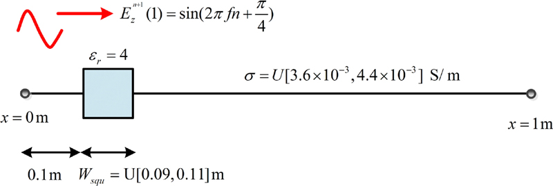
Figure 1: The calculating example of one-dimensional electromagnetic wave propagation.

The total length of the calculation example is 1 m, and there is a dielectric block starting at x = 0.1 m. There is uncertainty in the length of the dielectric block, which is a uniform distribution in the range of [0.09,0.11] m. The dielectric constant of the block is different from other regions, and the relative dielectric constant of other regions is 1, which is the same as the vacuum dielectric constant ${\epsilon }_0=8.8542\times {10}^{-12}\mathrm{F}/\mathrm{m}$. The relative dielectric constant of the dielectric block is 4, which is $\epsilon =4\times {\epsilon }_0$. The end position of the dielectric block can be modeled by the following random variable:

$$W_{\text{pocition}}\left({\xi }_1\right)=0.2+0.01\times {\xi }_1[\mathrm{m}].$$

(1)

${\xi }_1$ is a random variable with a uniform distribution in the range of $[-1,1]$.

The entire area, including the dielectric block, has the same permeability and conductivity. The value of the permeability is $\mu =4.0\times \pi \times {10}^{-7}\mathrm{H}/\mathrm{m}$, and the conductivity is an uncertain parameter $\sigma =U[3.6\times {10}^{-3},4.4\times {10}^{-3}]\mathrm{S}/\mathrm{m}$ with a uniform distribution:

$$\sigma \left({\xi }_2\right)=4\times {10}^{-3}\times \left(1+0.1{\xi }_2\right)[\mathrm{S}/\mathrm{m}].$$

(2)

${\xi }_2$ is also a random variable with a uniform distribution in the range of $[-1,1]$.

There is a sinusoidal excitation source of electric field strength at x = 0 m, and its expression is $\sin \left(2\pi fn+\frac{\pi }{4}\right)\mathrm{V}/\mathrm{m}$. Applying the finite difference time domain (FDTD), the space is discretized into 200 discrete points, that is, the space step is $\mathrm{\Delta }x=0.005\mathrm{m}$. In order to meet the Courant stability condition, the time step is calculated by the following formula:

$$\mathrm{\Delta }t=\frac{\mathrm{\Delta }x}{2\times c}=8.33\times {10}^{-12}\mathrm{s},$$

(3)

where c is the speed of light and its value is $3\times {10}^8\mathrm{m}/\mathrm{s}$. In this example, the simulation requires 2000 steps, so the total time of electromagnetic wave propagation is $T=2000\mathrm{\Delta }t=1.67\times {10}^{-8}\mathrm{s}$. The simulation result is the electric field intensity value of the entire area at time $T$.

It is worth noting that geometric uncertainty causes the randomness of material properties at different positions, and the corresponding relationship is presented as follows:

$${\epsilon }_r({\xi }_1,i)=\{\begin{array}{cc}1,\hfill & \hfill 1\le i\le 20\text{or}43\le i\le 200\\ 4,\hfill & \hfill 21\le i\le 37,\\ F\left({\xi }_1\right),\hfill & \hfill 38\le i\le 42\end{array}$$

(4)

where i indicates the location of discrete points, and $F\left({\xi }_1\right)$ is an unknown constant between 1 and 4.

The set of all random variables can describe the uncertainty factor of the model:

$$\xi =\{{\xi }_1,{\xi }_2\}.$$

(5)

After considering the random variable model in (5), one-dimensional random Maxwell equations can be represented:

$$\frac{\partial H_y(\xi )}{\partial t}=\frac{1}{\mu }\left(\frac{\partial E_z(\xi )}{\partial x}\right),$$

(6)

$$\frac{\partial E_z(\xi )}{\partial t}=\frac{1}{\epsilon ({\xi }_1,i)}\left(\frac{\partial H_y(\xi )}{\partial x}-\sigma \left({\xi }_2\right)E_z(\xi )\right).$$

(7)

The uncertainty in the simulation input is reflected in the parameters $\epsilon ({\xi }_1,i)$ and $\sigma \left({\xi }_2\right)$. This uncertainty will affect the output results through the simulation process, making it the function of $\xi$, together with electric field strength $E_z(\xi )$ and magnetic field strength $H_y(\xi )$.

After FDTD transformation [16, 17], the discrete of space and time is realized:

		$E_z^{n+1}(i,\xi )=\alpha (\xi ,i)E_z^n(i,\xi )+\beta (\xi ,i)$		(8)
		$\left[H_y^{n+1/2}(i+1/2,\xi )-H_y^{n+1/2}(i-1/2,\xi )\right],$

		$H_y^{n+1/2}(i+1/2,\xi )=H_y^{n-1/2}(i+1/2,\xi )$		(9)
		$+\gamma \left(E_z^n(i+1,\xi )-E_z^n(i,\xi )\right).$

The intermediate parameters can be expressed as:

$$\{\begin{array}{c}\hfill \alpha (\xi ,i)=\frac{1-\mathrm{\Delta }t\sigma \left({\xi }_2\right)/2\epsilon ({\xi }_1,i)}{1+\mathrm{\Delta }t\sigma \left({\xi }_2\right)/2\epsilon ({\xi }_1,i)}\hfill \\ \hfill \beta (\xi ,i)=\frac{\mathrm{\Delta }t}{\mathrm{\Delta }x\epsilon ({\xi }_1,i)\left[1+\mathrm{\Delta }t\sigma \left({\xi }_2\right)/2\epsilon ({\xi }_1,i)\right]}.\hfill \\ \hfill \gamma =\frac{\mathrm{\Delta }t}{\mu \mathrm{\Delta }x}\hfill \end{array}$$

(10)

The discrete one-dimensional Maxwell equations with random variables are shown. Then, how to solve these equations based on the SGM will be provided in next section.

III. UNCERTAINTY SIMULATION BASED ON THE SGM

The chaotic polynomial is used to expand the simulation outputs in formula (8). For convenience, we only take the first three polynomials as examples.

		$E_z^{n+1}(i,\xi )=e_0^{n+1,i}{\phi }_0(\xi )+$		(11)
		$e_1^{n+1,i}{\phi }_1(\xi )+e_2^{n+1,i}{\phi }_2(\xi ),$

$$E_z^n(i,\xi )=e_0^{n,i}{\phi }_0(\xi )+e_1^{n,i}{\phi }_1(\xi )+e_2^{n,i}{\phi }_2(\xi ),$$

(12)

		$H_y^{n+1/2}(i+1/2,\xi )=h_0^{n+1/2,i+1/2}{\phi }_0(\xi )+$		(13)
		$h_1^{n+1/2,i+1/2}{\phi }_1(\xi )+h_2^{n+1/2,i+1/2}{\phi }_2(\xi ),$

		$H_y^{n+1/2}(i-1/2,\xi )=h_0^{n+1/2,i-1/2}{\phi }_0(\xi )+$		(14)
		$h_1^{n+1/2,i-1/2}{\phi }_1(\xi )+h_2^{n+1/2,i-1/2}{\phi }_2(\xi ).$

Among them, ${\phi }_0(\xi )$, ${\phi }_1(\xi )$, and ${\phi }_2(\xi )$ are the chaotic polynomials, the coefficients in front of them are the parameters to be solved. According to the Askey rule, there is a one-to-one correspondence between random variables and chaotic polynomials [6]. The random variable with uniform distribution corresponds to the Legendre chaotic polynomial, and the result of the polynomial under one-dimensional random variable ${\xi }_i$ is proposed as

$${\phi }_0\left({\xi }_i\right)=1,$$

(15)

$${\phi }_1\left({\xi }_i\right)=\sqrt{3}{\xi }_i,$$

(16)

$${\phi }_2\left({\xi }_i\right)=\frac{\sqrt{5}}{2}\left(3{\xi }_i^2-1\right),$$

(17)

$${\phi }_3\left({\xi }_i\right)=\frac{\sqrt{7}}{2}\left(5{\xi }_i^3-3{\xi }_i\right).$$

(18)

In the example given in this article, the number of random variables is 2, so the corresponding chaotic polynomial form is presented in Table 1.

Table 1: Legendre polynomial under 2 variables

Expansion	Expansion	Legendre
Items	Order	Polynomial
0	0	1
1	1	$\sqrt{3}{\xi }_1$
2	1	$\sqrt{3}{\xi }_2$
3	2	$\frac{\sqrt{5}}{2}\left(3{\xi }_1^2-1\right)$
4	2	$3{\xi }_1{\xi }_2$
5	2	$\frac{\sqrt{5}}{2}\left(3{\xi }_2^2-1\right)$
6	3	$\frac{\sqrt{7}}{2}\left(5{\xi }_1^3-3{\xi }_1\right)$
7	3	$\frac{\sqrt{15}}{2}\left(3{\xi }_1^2-1\right){\xi }_2$
8	3	$\frac{\sqrt{15}}{2}\left(3{\xi }_2^2-1\right){\xi }_1$
9	3	$\frac{\sqrt{7}}{2}\left(5{\xi }_2^3-3{\xi }_2\right)$

The chaotic polynomials are orthogonal to each other, and the mathematical description is:

$$⟨{\phi }_i,{\phi }_j⟩=⟨{\phi }_i^2⟩{\delta }_{ij},$$

(19)

$${\delta }_{ij}=\{\begin{array}{cc}1\hfill & (i=j)\hfill \\ 0\hfill & (i\ne j)\hfill \end{array}.$$

(20)

The inner product calculation is defined as

$$⟨{\phi }_i,{\phi }_j⟩=\int {\phi }_i(\xi ){\phi }_j(\xi )w(\xi )\mathit{d}\xi .$$

(21)

Among them, $w(\xi )$ is the weight function, which is the joint probability density function of all random variables. When all random variables are independent of one another, $w(\xi )$ can be calculated by directly multiplying the probability density functions of each random variable. The integral operation in the formula is a multiple definite integral operation. The integral multiplicity is the number of random variables in the random space. The upper and lower limits of the integral are hypercubes composed of the upper and lower limits of each random variable.

After putting formulas (11) to (14) into formula (8), and then applying ${\phi }_0(\xi )$ to do the inner product operation on both sides of the equation, the following equation can be provided:

		$e_0^{n+1,i}=e_0^{n,i}⟨\alpha (\xi ,i){\phi }_0(\xi ),{\phi }_0(\xi )⟩$		(22)
		$+e_1^{n,i}⟨\alpha (\xi ,i){\phi }_1(\xi ),{\phi }_0(\xi )⟩+e_2^{n,i}⟨\alpha (\xi ,i){\phi }_2(\xi ),{\phi }_0(\xi )⟩$
		$+\left(h_0^{n+1/2,i+1/2}-h_0^{n+1/2,i-1/2}\right)⟨\beta (\xi ,i){\phi }_0(\xi ),{\phi }_0(\xi )⟩$
		$+\left(h_1^{n+1/2,i+1/2}-h_1^{n+1/2,i-1/2}\right)⟨\beta (\xi ,i){\phi }_1(\xi ),{\phi }_0(\xi )⟩$
		$+\left(h_2^{n+1/2,i+1/2}-h_2^{n+1/2,i-1/2}\right)⟨\beta (\xi ,i){\phi }_2(\xi ),{\phi }_0(\xi )⟩.$

In the same way, the following equations can be arranged by performing inner product operations with ${\phi }_1(\xi )$ and ${\phi }_2(\xi )$ respectively:

		$\left[\begin{array}{c}{e}_0^{n+1,i}\hfill \\ e_1^{n+1,i}\hfill \\ e_2^{n+1,i}\hfill \end{array}\right]=\left[\begin{array}{ccc}{A}_{0,0}^{\alpha ,i}\hfill & A_{1,0}^{\alpha ,i}\hfill & A_{2,0}^{\alpha ,i}\hfill \\ A_{0,1}^{\alpha ,i}\hfill & A_{1,1}^{\alpha ,i}\hfill & A_{2,1}^{\alpha ,i}\hfill \\ A_{0,2}^{\alpha ,i}\hfill & A_{1,2}^{\alpha ,i}\hfill & A_{2,i}^{\alpha ,i}\hfill \end{array}\right]\left[\begin{array}{c}\hfill e_0^{n,i}\hfill \\ \hfill e_1^{n,i}\hfill \\ \hfill e_2^{n,i}\hfill \end{array}\right]+$		(23)
		$\left[\begin{array}{ccc}{A}_{0,0}^{\beta ,i}\hfill & A_{1,0}^{\beta ,i}\hfill & A_{2,0}^{\beta ,i}\hfill \\ A_{0,1}^{\beta ,i}\hfill & A_{1,1}^{\beta ,i}\hfill & A_{2,1}^{\beta ,i}\hfill \\ A_{0,2}^{\beta ,i}\hfill & A_{1,2}^{\beta ,i}\hfill & A_{2,2}^{\beta ,i}\hfill \end{array}\right]\times \left[\begin{array}{c}{h}_0^{n+1/2,i+1/2}-h_0^{n+1/2,i-1/2}\hfill \\ h_1^{n+1/2,i+1/2}-h_1^{n+1/2,i-1/2}\hfill \\ h_2^{n+1/2,i+1/2}-h_2^{n+1/2,i-1/2}\hfill \end{array}\right].$

Among them, the middle parameter represents the inner product operation process:

$$\{\begin{array}{c}{A}_{m,l}^{\alpha ,i}=⟨\alpha (\xi ,i){\phi }_m(\xi ),{\phi }_l(\xi )⟩\hfill \\ A_{m,l}^{\beta ,i}=⟨\beta (\xi ,i){\phi }_m(\xi ),{\phi }_l(\xi )⟩\hfill \end{array}\mathit{\hspace{1em}}m,l=0,1,2.$$

(24)

As shown in formula (4), due to geometric uncertainty, the inner product calculation formula at each discrete point is different, the calculation formula is calculated as follows:

		$⟨\alpha (\xi ,i){\phi }_{xi}(\xi ),{\phi }_{yi}(\xi )⟩=$		(25)
		$\{\begin{array}{c}\hfill {\displaystyle \frac{1}{4}}{\displaystyle {\int }_{-1}^1}{\displaystyle {\int }_{-1}^1}{\displaystyle \frac{1-\mathrm{\Delta }t\sigma \left({\xi }_2\right)/2{\epsilon }_0}{1+\mathrm{\Delta }t\sigma \left({\xi }_2\right)/2{\epsilon }_0}}{\phi }_{xi}(\xi ){\phi }_{yi}(\xi )\mathit{d}{\xi }_1\mathit{d}{\xi }_2\hfill \\ \hfill 1\le i\le 20\text{or}43\le i\le 200\hfill \\ \hfill Q_{\alpha },38\le i\le 42\hfill \\ \hfill {\displaystyle \frac{1}{4}}{\displaystyle {\int }_{-1}^1}{\displaystyle {\int }_{-1}^1}{\displaystyle \frac{1-\mathrm{\Delta }t\sigma \left({\xi }_2\right)/8{\epsilon }_0}{1+\mathrm{\Delta }t\sigma \left({\xi }_2\right)/8{\epsilon }_0}}{\phi }_{xi}(\xi ){\phi }_{yi}(\xi )\mathit{d}{\xi }_1\mathit{d}{\xi }_2\hfill \\ \hfill 21\le i\le 37,\hfill \end{array}$

		$Q_{\alpha }=$		(26)
		${\displaystyle \frac{1}{4}}{\displaystyle {\int }_{-1}^1}{\displaystyle {\int }_{-1}^{\frac{i/40-1}{0.05}}}{\displaystyle \frac{1-\mathrm{\Delta }t\sigma \left({\xi }_2\right)/2{\epsilon }_0}{1+\mathrm{\Delta }t\sigma \left({\xi }_2\right)/2{\epsilon }_0}}{\phi }_{xi}(\xi ){\phi }_{yi}(\xi )\mathit{d}{\xi }_1\mathit{d}{\xi }_2+$
		${\displaystyle \frac{1}{4}}{\displaystyle {\int }_{-1}^1}{\displaystyle {\int }_{\frac{i/40-1}{0.1}}^1}{\displaystyle \frac{1-\mathrm{\Delta }t\sigma \left({\xi }_2\right)/8{\epsilon }_0}{1+\mathrm{\Delta }t\sigma \left({\xi }_2\right)/8{\epsilon }_0}}{\phi }_{xi}(\xi ){\phi }_{yi}(\xi )\mathit{d}{\xi }_1\mathit{d}{\xi }_2,$

		$⟨\beta (\xi ,i){\phi }_{xi}\left(\xi \right),{\phi }_{yi}\left(\xi \right)⟩$		(27)
		$=\{\begin{array}{c}{\displaystyle \frac{1}{4}}{\displaystyle {\int }_{-1}^1}{\displaystyle {\int }_{-1}^1}{\displaystyle \frac{\mathrm{\Delta }t}{\mathrm{\Delta }x{\epsilon }_0\left[1+\mathrm{\Delta }t\sigma \left({\xi }_2\right)/2{\epsilon }_0\right]}}{\phi }_{xi}\left(\xi \right){\phi }_{yi}\left(\xi \right)\mathit{d}{\xi }_1\mathit{d}{\xi }_2\hfill \\ 1\le i\le 20\text{or}43\le i\le 200\hfill \\ Q_{\beta },38\le i\le 42\hfill \\ {\displaystyle \frac{1}{4}}{\displaystyle {\int }_{-1}^1}{\displaystyle {\int }_{-1}^1}{\displaystyle \frac{\mathrm{\Delta }t}{4\mathrm{\Delta }x{\epsilon }_0\left[1+\mathrm{\Delta }t\sigma \left({\xi }_2\right)/8{\epsilon }_0\right]}}{\phi }_{xi}\left(\xi \right){\phi }_{yi}\left(\xi \right)\mathit{d}{\xi }_1\mathit{d}{\xi }_2\hfill \\ 21\le i\le 37,\hfill \end{array}$

		$Q_{\beta }=$		(28)
		${\displaystyle \frac{1}{4}}{\displaystyle {\int }_{-1}^1}{\displaystyle {\int }_{-1}^{\frac{i/40-1}{0.05}}}{\displaystyle \frac{\mathrm{\Delta }t}{\mathrm{\Delta }x{\epsilon }_0\left[1+\mathrm{\Delta }t\sigma \left({\xi }_2\right)/2{\epsilon }_0\right]}}$
		${\phi }_{xi}\left(\xi \right){\phi }_{yi}\left(\xi \right)d{\xi }_{1}d{\xi }_2+$
		${\displaystyle \frac{1}{4}}{\displaystyle {\int }_{-1}^1}{\displaystyle {\int }_{\frac{i/40-1}{0.05}}^1}{\displaystyle \frac{\mathrm{\Delta }t}{4\mathrm{\Delta }x{\epsilon }_0\left[1+\mathrm{\Delta }t\sigma \left({\xi }_2\right)/8{\epsilon }_0\right]}}$
		${\phi }_{xi}\left(\xi \right){\phi }_{yi}\left(\xi \right)d{\xi }_{1}d{\xi }_2.$

Among them, the calculation process of the boundary point $\frac{i/40-1}{0.05}$ of the integral limit is provided as follows:

$$W_{\text{position}}\left({\xi }_{1,\text{lim}}\right)=40\mathrm{\Delta }x\left(1+0.05{\xi }_{1,\text{lim}}\right),$$

(29)

$$W_{\text{position}}\left({\xi }_{1,lim}\right)=i\mathrm{\Delta }x,$$

(30)

$$i\mathrm{\Delta }x=40\mathrm{\Delta }x\left(1+0.05{\xi }_{1,\text{lim}}\right),$$

(31)

$${\xi }_{1,lim}=\frac{i/40-1}{0.05}.$$

(32)

The SGM transforms the stochastic Maxwell equations shown in equation (8) into the augmented deterministic Maxwell equations shown in equation (23). Next, the traditional FDTD method can be used to solve equation (23) to obtain the chaotic polynomial coefficients in equations (11) to (14). Finally, by statistical sampling of random variables, the final uncertainty analysis results can be obtained, such as expectation value, standard deviation, worst-case estimate, probability density curve, and so on.

IV. SIMULATION RESULT OF THE SGM AND ITS VALIDITY ANALYSIS

Figure 2 shows the expectation value results of electric field intensity at each discrete point based on the SGM, and Fig. 3 shows the corresponding standard deviation results. Simulation results of the MCM are also given as standard data.

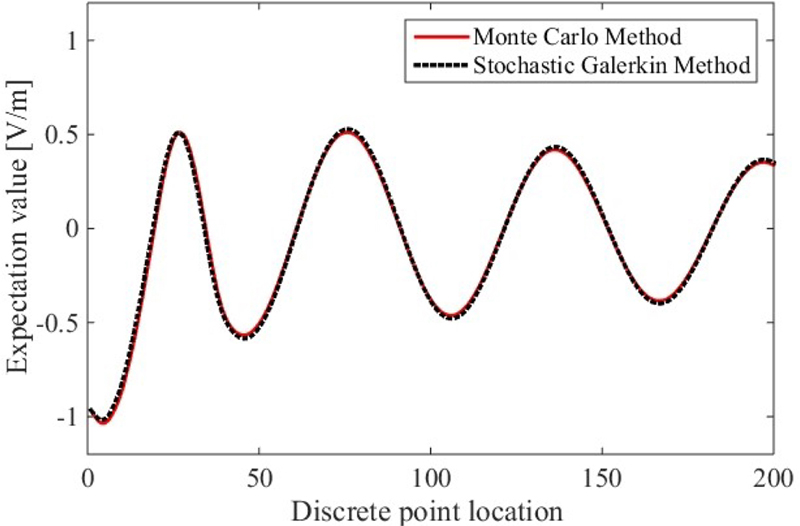
Figure 2: Comparison of expectation values between the SGM and the MCM.

Feature selective validation (FSV) method [18, 19] is used to compare the difference between two sets of one-dimensional curves. In Fig. 2, the FSV value between the MCM and the SGM in expectation value results is 0.04, and it is presented that the accuracy of the SGM is in “Excellent” level. In Fig. 3, the FSV value is 0.25, and it is shown that the accuracy of the SGM in standard deviation results is only in “Good” level. It is clearly seen that there is a significant difference between the two curves in Fig. 3.

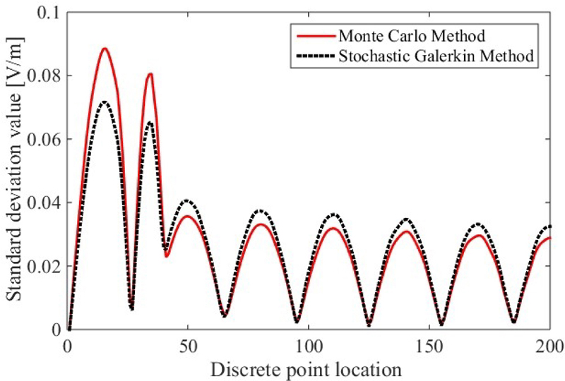
Figure 3: Comparison of standard deviations between the SGM and the MCM.

Back to equation (4), since $F\left({\xi }_1\right)$ is an unknown random number, the following inner product calculation formula is needed to deal with this geometric uncertainty:

		${\displaystyle {\int }_{-1}^1}f\left({\epsilon }_r({\xi }_1,i)\right)\mathit{d}{\xi }_1={\displaystyle {\int }_{-1}^1}f\left(F\left({\xi }_1\right)\right)\mathit{d}{\xi }_1$		(33)
		$\approx {\displaystyle {\int }_{-1}^{\frac{i/40-1}{0.05}}}f(4)\mathit{d}{\xi }_1+$
		${\displaystyle {\int }_{\frac{i/40-1}{0.05}}^1}f(1)\mathit{d}{\xi }_1,i=38,\mathrm{\dots },42.$

Both equation (26) and equation (28) are derived from the principle shown in equation (33). Figure 4 is given in order to better demonstrate its mathematical principle. It is shown that the area of the curved trapezoid below the red dotted line is approximately equal to the sum of the areas of the two rectangles. This is the principle of numerical integration calculation.

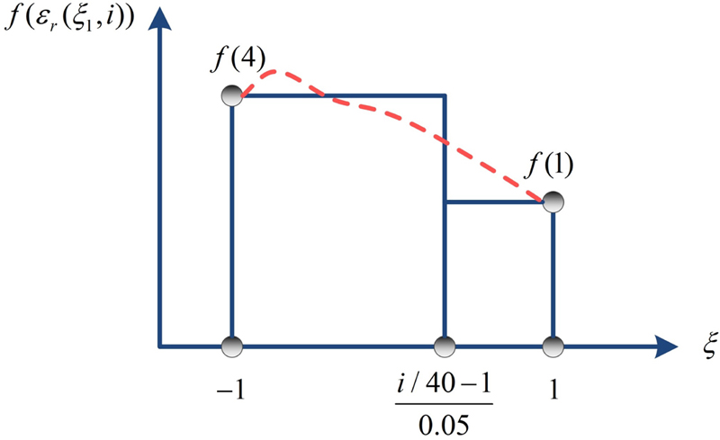
Figure 4: Mathematical principle of numerical integration calculation.

This approximate calculation is right, but additional error will ensue. For under normal conditions, the error in the SGM is caused solely by the truncation of chaotic polynomials. However, in this calculation example, there is not only truncation error, but also additional error caused by numerical integration operations. Therefore, the introduction of additional error is the reason why the SGM fails.

V. UNCERTAINTY SIMULATION BASED ON THE SCM

The uncertainty simulation based on the SCM is given in this section as a comparison. Zero points of the chaotic polynomial are selected as the collocation points of the SCM. According to numerical analysis theory, these zero points are Gaussian volume points, which can maximize the convergence of the algorithm and thus improve its computational accuracy [12, 14]. For example, the collocation points in the case of one-dimensional and three-order polynomial (17) is $\{0,\pm \frac{\sqrt{15}}{5}\}$. In this paper, the calculation example contains two random variables, and the collocation points are given in the form of tensor product ${\mathrm{P}}_{SCM}=\{0,\pm \frac{\sqrt{15}}{5}\}\otimes \{0,\pm \frac{\sqrt{15}}{5}\}$. Performing the multi-dimensional Lagrange interpolation algorithm on the collocation points, the uncertainty analysis results of the SCM can be obtained:

		${\mathrm{EMC}}_{\mathrm{SCM}}(\xi )=$		(34)
		${\displaystyle \sum _{j_1=1}^3}{\displaystyle \sum _{j_2=1}^3}\mathrm{EMC}\left({\mathrm{P}}_{SCM}\right)\times \mathrm{Lag}({\mathrm{P}}_{SCM},\xi ).$

$\xi$ still represents a collection of random variables $\{{\xi }_1,{\xi }_2\}$. $\mathrm{EMC}\left({\mathrm{P}}_{SCM}\right)$ refers to the deterministic EMC simulation result at the collocation points. $\mathrm{Lag}({\mathrm{P}}_{SCM},\xi )$ refers to the multidimensional Lagrange interpolation results at the collocation points, and it is a function of the random variable $\xi$.

Finally, statistical sampling is also required, and the final uncertainty analysis results can be obtained.

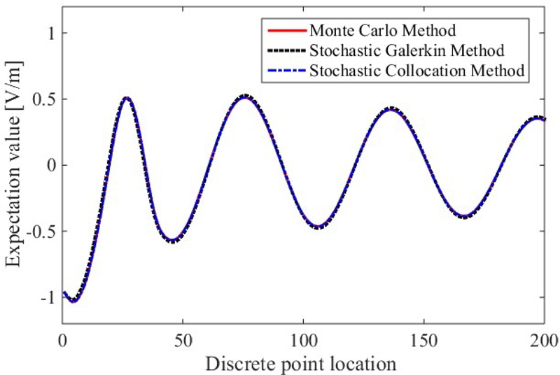
Figure 5: Expectation values provided by the SCM.

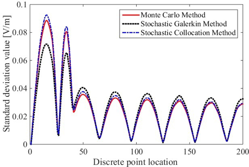
Figure 6: Standard deviations provided by the SCM.

The uncertainty analysis based on the SCM is performed on the calculating example in Fig. 1, the results of expectation values and standard deviations are provided in Figs. 5 and 6, respectively. Using the FSV method, the FSV value between the MCM and the SCM in expectation value results is 0.03, and the value in standard deviation results is 0.07. Compared with FSV values of SGM, both 0.03 and 0.04 belong to the range of greater than 0 but less than 0.1, which belongs to the “Excellent” level in the qualitative judgment criteria for FSV. However, the difference between 0.03 and 0.04 is not significant, and it can be considered that the accuracy of the expected values for the SCM and the SGM is very similar. Looking at the standard deviation results in Fig. 6, it is evident from the figures that the accuracy of the SCM is much higher than that of the SGM. From the perspective of FSV value, the SCM’s FSV value of 0.07 still belongs to the “Excellent” level, while the SGM’s 0.25 is only the “Good” level, which differs by two levels in qualitative standards. In summary, in this calculation example, the calculation accuracy of the SCM is much higher than that of the SGM, which is at the same level of accuracyas the MCM.

The SCM is a non-embedded uncertainty analysis method and will not modify the original solver. Therefore, there is only truncation error of the chaotic polynomial in the SCM simulation results and no additional error introduced by the numerical integration. Conversely, the SGM contains two types of errors (its principle has been explained in Fig. 4), so the theoretical accuracy of the SGM in this example is lower than that of the SCM. Obviously, in this calculating example, the SCM is more accurate than the SGM. Therefore, the reliability of the SCM is much higher than that of the SGM, and only a stable and reliable deterministic EMC solver is needed. At the same time, the programming implementation of the SCM is much easier than the SGM, and it can effectively avoid calculation accuracy deviations caused by programming errors.

The simulation time of the MCM is 1.17 hours, and that of the SGM is 0.10 hours, but that of the SCM is only 5.16 seconds. Because the MCM is based on the law of weak large numbers, a large number of deterministic EMC simulations are needed to ensure convergence, so the simulation time is the longest. The SGM needs to calculate the numerical integration at different discrete points, so it also takes a certain amount of time for simulation. The SCM takes the shortest time since it only needs 9 deterministic EMC simulations.

It is worth noting that the single EMC simulation time of this example is relatively short, so the time of numerical integration calculation appears relatively long. As a result, the calculation efficiency of the SCM is better than that of the SGM. However, when the single simulation time is much longer than the numerical integration time, the calculation efficiency of the SGM and the SCM are at the same level. Of course, their computational efficiency is far better than the MCM under any conditions.

VI. CONCLUSION

After properly taking geometric uncertainty into consideration, this paper, aiming at a published example of a typical EMC simulation, found that the results of uncertainty analysis of the SGM are far from expected, which means the error of the SGM was hard to ignore. According to failure mechanism, the root cause of the failure of the simulation is the additional error introduced by using numerical integration to solve the inner product formula. Compared with the results of the SCM, it’s concluded that the SCM is more accurate than the SGM when processing geometric uncertaintyfactors.

Through analysis of the failure mechanism, the applicable scope of the SGM was further determined, thus general selective strategies of uncertainty analysis method should be rectified: (1) the MCM should be adopted when the time of a single simulation is relatively short; (2) the SGM should be selected when a model has long single simulation time, high computational accuracy demand, and its solver is easy to change without modifying the inner product formula; (3) the SCM is to be preferred in any other situation that hasn’t been mentioned above.

ACKNOWLEDGMENT

This work was supported in part by the Youth Science Foundation Project, National Natural Science Foundation of China, under Grant 52301414.

REFERENCES

[1] S. A. Pignari, S. Giordano, and G. Flavia, “Modeling field-to-wire coupling in random bundles of wires,” IEEE Electromagnetic Compatibility Magazine, vol. 6, no. 3, pp. 85-90, Nov. 2017.

[2] H. Xie, J. F. Dawson, J. Yan, A. C. Marvin, and M. P. Robinson, “Numerical and analytical analysis of stochastic electromagnetic fields coupling to a printed circuit board trace,” IEEE Transactions on Electromagnetic Compatibility, vol. 62, no. 4, pp. 1128-1135, Aug. 2020.

[3] Y. Zhang, C. Liao, R. Huan, Y. Shang, and H. Zhou, “Analysis of nonuniform transmission lines with a perturbation technique in time domain,” IEEE Transactions on Electromagnetic Compatibility, vol. 62, no. 2, pp. 542-548, April 2020.

[4] A. Gillman, A. H. Barnett, and P.-G. Martinsson, “A spectrally accurate direct solution technique for frequency domain scattering problems with variable media,” BIT Numerical Mathematics, vol. 55, no. 1, pp. 141-170, Aug. 2013.

[5] J. Bai, G. Zhang, L. Wang, and T. Wang, “Uncertainty analysis in EMC simulation based on improved method of moments,” Applied Computational Electromagnetics Society Journal, vol. 31, no. 1, pp. 66-71, Jan. 2016.

[6] R. Edwards, A. Marvin, and S. Porter, “Uncertainty analyses in the finite difference time domain method,” IEEE Transactions on Electromagnetic Compatibility, vol. 52, no. 1, pp. 155-163, Feb. 2010.

[7] Z. Fei, Y. Huang, J. Zhou, and Q. Xu, “Uncertainty quantification of crosstalk using stochastic reduced order models,” IEEE Transactions on Electromagnetic Compatibility, vol. 59, no. 1, pp. 228-239, Feb. 2016.

[8] P. Manfredi, D. V. Ginste, I. S. Stievano, D. De Zutter, and F. G. Canavero, “Stochastic transmission line analysis via polynomial chaos methods: An overview,” IEEE Electromagnetic Compatibility Magazine, vol. 6, no. 3, pp. 77-84, Nov. 2017.

[9] P. Manfredi, D. V. Ginste, D. De Zutter, and F. G. Canavero, “Generalized decoupled polynomial chaos for nonlinear circuits with many random parameters,” IEEE Microwave & Wireless Components Letters, vol. 25, no. 8, pp. 505-507, Aug. 2015.

[10] P. Manfredi, R. Trinchero, and D. V. Ginste, “A perturbative stochastic Galerkin method for the uncertainty quantification of linear circuits,” IEEE Transactions on Circuits and Systems, vol. 67, no. 9, pp. 2993-3006, 2020.

[11] T.-L. Wu, F. Buesink, and F. Canavero, “Overview of signal integrity and EMC design technologies on PCB: Fundamentals and latest progress,” IEEE Transactions on Electromagnetic Compatibility, vol. 55, no. 4, pp. 624-638, Aug. 2013.

[12] B. Xia, Y. Chen, W. Yang, Q. Chen, X. Wang, and K. Min, “Stochastic optimal power flow for power systems considering wind farms based on the stochastic collocation method,” IEEE Access, vol. 10, no. 1, pp. 44023-44032, April 2022.

[13] Y. Chi, B. Li, X. Yang, T. Wang, K. Yang, and Y. Gao, “Research on the statistical characteristics of crosstalk in naval ships wiring harness based on polynomial chaos expansion method,” Polish Maritime Research, vol. 24, no. s2, pp. 205-214, Aug. 2017.

[14] J. Bai, G. Zhang, D. Wang, A. P. Duffy, and L. Wang, “Performance comparison of the SGM and the SCM in EMC simulation,” IEEE Transactions on Electromagnetic Compatibility, vol. 58, no. 6, pp. 1739-1746, Dec. 2016.

[15] J. Bai, G. Zhang, L. Wang, and D. Alistair, “Uncertainty analysis in EMC simulation based on stochastic collocation method,” IEEE Electromagnetic Compatibility Magazine, pp. 930-934, Sep. 2015.

[16] M. Moradi, V. Nayyeri, S.-M. Sadrpour, M. Soleimani, and O. M. Ramahi, “A 3-D weakly conditionally stable single-field finite-difference time-domain method,” IEEE Transactions on Electromagnetic Compatibility, vol. 62, no. 2, pp. 498-509, April 2020.

[17] R. Tsuge, Y. Baba, H. Kawamura, and N. Itamoto, “Finite-difference time-domain simulation of a lightning-impulse-applied ZnO element,” IEEE Transactions on Electromagnetic Compatibility, vol. 62, no. 5, pp. 1780-1786, Oct. 2020.

[18] A. P. Duffy, A. Orlandi, and Z. Gang, “Review of the feature selective validation method (FSV). Part I-Theory,” IEEE Transactions on Electromagnetic Compatibility, vol. 60, no. 4, pp. 814-821, Aug. 2018.

[19] A. Orlandi, A. P. Duffy, and Z. Gang, “Review of the feature selective validation method (FSV). Part II-Performance analysis and research fronts,” IEEE Transactions on Electromagnetic Compatibility, vol. 60, no. 4, pp. 1029-1035, Aug. 2018.

BIOGRAPHIES

Jinjun Bai received the Ph.D. degree in electrical engineering in 2019 from the Harbin Institute of Technology, Harbin, China. He is now a lecturer at Dalian Maritime University. His research interests include uncertainty analysis methods in EMC simulation.

Bing Hu He is currently a graduate student in electrical engineering at Dalian Maritime University, where his research interests include uncertainty analysis methods in EMC simulation.

Yixuan Wan She is working toward a master’s degree in electrical engineering. Her current research on simulation of electromagnetic radiation related to electric vehicles. She is now engaged in electric vehicle cable harness crosstalk simulation.

ACES JOURNAL, Vol. 38, No. 7, 475–481
doi: 10.13052/2023.ACES.J.380702
© 2023 River Publishers

ABSTRACT

I. INTRODUCTION

II. CALCULATION EXAMPLE CONSIDERING GEOMETRIC UNCERTAINTY

III. UNCERTAINTY SIMULATION BASED ON THE SGM

IV. SIMULATION RESULT OF THE SGM AND ITS VALIDITY ANALYSIS

V. UNCERTAINTY SIMULATION BASED ON THE SCM

VI. CONCLUSION

ACKNOWLEDGMENT

REFERENCES

BIOGRAPHIES