Shaping the Probability Density Function of the Output Response in a Reverberation Chamber

Qian Xu${}^{\mathbf{\text{1}}}$, Feng Tian${}^{\mathbf{\text{1}}}$, Yongjiu Zhao${}^{\mathbf{\text{1}}}$, Rui Jia${}^{\mathbf{\text{2}}}$, Erwei Cheng${}^{\mathbf{\text{3}}}$, and Lei Xing${}^{\mathbf{\text{1}}}$

¹College of Electronic and Information Engineering
Nanjing University of Aeronautics and Astronautics, Nanjing 211106, China
emxu@foxmail.com, yjzhao@nuaa.edu.cn, emxinglei@foxmail.com

²State Key Laboratory of Complex Electromagnetic Environment Effects on Electronic and Information System Luo Yang 471003, China
jiarui315@163.com

³Department of Engineering Physics, Tsinghua University, Beijing
China and National Key Laboratory on Electromagnetic Environment Effects
Army Engineering University Shijiazhuang Campus, Shijiazhuang 050004, China
ew_cheng@163.com

Submitted On: January 10, 2023; Accepted On: April 24, 2023

ABSTRACT

This paper shows that the received power and E-field in a reverberation chamber (RC) can be shaped by tuning the statistical properties of input signals. For a given probability density function (PDF) of an RC response, the Fourier transform method can be applied to find the PDF of the input signal. Numerical and measurement verifications are given to validate the theory. Limitations are also analyzed and discussed.

Index Terms: probability density function, reverberation chamber.

I. INTRODUCTION

A reverberation chamber (RC) is a highly resonant electrically large cavity which is equipped with mechanical stirrers inside (Fig. 1 (a)). The stirrers are used to tune the boundary conditions inside the cavity to generate statistically isotropic and uniform electromagnetic fields. In recent years, RCs have been widely used in electromagnetic compatibility (EMC) and over-the-air (OTA) testing [1, 2]. Unlike an anechoic chamber which is designed as a deterministic system, an RC was born to be a statistical environment. It has been found that for a well-stirred RC, the received power has an exponential distribution and the magnitude of the rectangular E-field component ($\left|E_x\right|,\left|E_y\right|$ or $\left|E_z\right|$) has a Rayleigh distribution [3]. In vehicles, ships and planes, when more cavities are cascaded or nested, the E-field magnitude may no longer be Rayleigh distribution.

Due to the inherent statistical properties of an RC, a Rayleigh distribution (or a Rician distribution) can be well emulated, and theK-factors can be tuned statistically [4–8]. By combining an RC with a channel emulator, a complex channel response can be emulated [9–11].

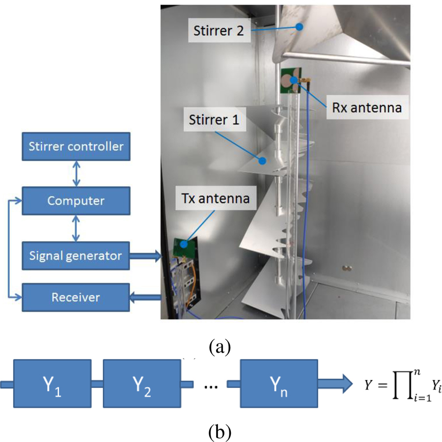
Figure 1: (a) Typical measurement setup in an RC; the inner dimensions are 0.94 m $\times$ 1.16 m $\times$ 1.44 m. (b) Multi-cavity coupling model.

However, it does not seem easy to emulate response with arbitrary statistical distributions. If more distribution functions are expected in the channel emulation, refined controls are necessary. This paper proposes a method to control the PDF of RC responses in the frequency domain (FD), which can be used for the emulation of multi-cavity statistics in a single RC instead of actually using multiple connected cavities.

In this paper, Section II presents the theory, Section III starts from a simplified scenario and demonstrates the product of two random variables analytically and experimentally. Limitations and generalizations to multi-cavity models are discussed in Section IV.

II. THEORY

In the FD, when an RC is well-stirred and the magnitude of the input signal is a constant, the magnitude of rectangular E-field ($\left|E_x\right|$) inside the RC has a Rayleigh distribution [3]:

$$p_Y\left(y\right)=y{e}^{-\frac{y^2}{2{\sigma }_y^2}}/{\sigma }_y^2,y=\left|E_x\right|,$$

(1)

of which the expected value and the standard deviation are ${\sigma }_y\sqrt{\pi /2}$ and ${\sigma }_y\sqrt{2-\pi /2}$, respectively. When the statistical property of the input signal can be controlled, the PDF of the RC response ($E_{\mathrm{out}}$) can be tuned. Generally, the product of two random variables $Z=X\times Y$ can be used to synthesize the output response of a system, where $X$, $Y$ and $Z$ are the input variable, transfer function and output variable, respectively. Thus, the problem can be mathematically described as: for the given PDFs of random variable $Z$ and $Y$, and $Z=X\times Y$, what is the PDF of random variable $X$?

A misleading procedure is to use $X=Z/Y$ to calculate the PDF of $X$, which is wrong. The result will depend on specific set of $Z$ and $Y$. This procedure can be understood from the Mellin transform: when using $X^{\prime }=Z/Y$, the Mellin transform of the PDF of random variable $X^{\prime }$ can be obtained as $M_Z\left(s\right)M_Y\left(2-s\right)=M_X(s)M_Y(s)M_Y\left(2-s\right)$ which is not equal to $M_X(s)$ (only when $M_Y\left(s\right)M_Y\left(2-s\right)=1$) [12]. To find the PDF of $X$, a direct method is to use the Mellin and inverse Mellin transform, the result can be obtained quickly as ${ℳ}^{-1}[M_Z\left(s\right)/M_Y(s)]$. However, the numerical Mellin and inverse Mellin transform are not easy to calculate. In this paper, we adopt an approach with Fourier transforms.

From $Z=X\times Y$, we have $\ln Z=\ln X+\ln Y$ when $X$ and $Y$ are positive. Suppose the PDF of $\ln Z$, $\ln X$ and $\ln Y$ are $p_{\mathrm{lnZ}}(z)$, $p_{\mathrm{lnX}}(x)$ and $p_{\mathrm{lnY}}(y)$, respectively. We have

$$H_{\mathrm{lnZ}}\left(j\omega \right)=H_{\mathrm{lnX}}\left(j\omega \right)H_{\mathrm{lnY}}\left(j\omega \right),$$

(2)

where $H_{\mathrm{lnZ}}\left(j\omega \right)$, $H_{\mathrm{lnX}}\left(j\omega \right)$ and $H_{\mathrm{lnY}}\left(j\omega \right)$ are the Fourier transforms of $p_{\mathrm{lnZ}}(z)$, $p_{\mathrm{lnX}}(x)$ and $p_{\mathrm{lnY}}(y)$, respectively. (e.g., $H_{\mathrm{lnX}}\left(j\omega \right)={\int }_{-\mathrm{\infty }}^{+\mathrm{\infty }}{p}_{\mathrm{lnX}}(x)e^{-j\omega x}dx$). Thus, the PDF of the input signal $p_{\mathrm{lnX}}(x)$ can be calculated by using the inverse Fourier transform

$$p_{\mathrm{lnX}}\left(x\right)={ℱ}^{-1}\left[H_{\mathrm{lnZ}}\left(j\omega \right)/H_{\mathrm{lnY}}\left(j\omega \right)\right].$$

(3)

Finally, by applying the variable transform $e^X$ to $\ln X$, the PDF of $X$ (in linear unit) can be obtained.

III. DERIVATIONS AND VERIFICATIONS

When two RCs are nested or contiguous [13], a double-Rayleigh PDF response can be obtained. Suppose we want to emulate a double-Rayleigh PDF response in a single RC. We can control the magnitude of the input signal to have a random excitation. Assume the magnitude of the input signal has a PDF of

$$p_{\mathrm{X}}\left(x\right)=x{e}^{-\frac{x^2}{2{\sigma }_x^2}}/{\sigma }_x^2,x=\left|E_{in}\right|,$$

(4)

and the RC has a transfer function ($Y$) given in (1), the PDF of the response has been obtained in [13] as

$$p_{\mathrm{Z}}\left(z\right)=\frac{z}{{\sigma }_x^2{\sigma }_y^2}{K}_0\left(\frac{z}{{\sigma }_x{\sigma }_y}\right),z=\left|E_{\mathrm{out}}\right|,$$

(5)

where $K_0(.)$ is the zero-order modified Bessel function of the second kind, and the expected value and the standard deviation of (5) are ${\sigma }_x{\sigma }_y\pi /2$ and ${\sigma }_x{\sigma }_y\sqrt{4-{\pi }^2/4}$, respectively. $\left|E_{in}\right|$ and $\left|E_{\mathrm{out}}\right|$ represent the magnitude of the input signal (E-field) and the output signal (E-field), respectively. From (4), the PDF of $\ln X$ can be obtained as

$$p_{\mathrm{lnX}}\left(x\right)=e^{2x}{e}^{-\frac{e^{2x}}{2{\sigma }_x^2}}/{\sigma }_x^2,x=\ln \left|E_{in}\right|,$$

(6)

of which the mean and the standard deviation are $\mathrm{ln2}/2+\ln {\sigma }_x-\gamma /2$ and $\pi \sqrt{6}/12$, respectively ($\gamma \approx 0.5772$ is the Euler-Mascheroni constant). The Fourier transform of (6) is

$$H_{\mathrm{lnX}}\left(j\omega \right)={\left(\sqrt{2}{\sigma }_x\right)}^{-j\omega }\mathrm{\Gamma }\left(1-j\omega /2\right).$$

(7)

The Fourier transform of $p_{\mathrm{lnY}}\left(y\right)$ is the same as (7) but ${\sigma }_x$ is replaced by ${\sigma }_y$. It can be verified that the Fourier transform of

$$p_{\mathrm{lnZ}}\left(z\right)=\frac{e^{2z}}{{\sigma }_x^2{\sigma }_y^2}{K}_0\left(\frac{e^z}{{\sigma }_x{\sigma }_y}\right),z=\ln \left|E_{\mathrm{out}}\right|,$$

(8)

is

$$H_{\mathrm{lnZ}}\left(j\omega \right)={\left(2{\sigma }_x{\sigma }_y\right)}^{-j\omega }{\mathrm{\Gamma }}^2\left(1-j\omega /2\right).$$

(9)

To verify this procedure numerically, Monte-Carlo simulations are performed with parameters ${\sigma }_x=1$ and ${\sigma }_y=4$. We solve the PDF of $X$ from $Z$ and $Y$ using the numerical method and compare the results with analytical expressions. ${10}^6$ samples of $X$ and $Y$ are generated with Rayleigh distributions. The output variable $Z=X\times Y$ can be obtained. The histograms of $\ln Z$ and $\ln Y$ are illustrated in Fig. 2 (a) with analytical expressions. The corresponding Fourier transforms are presented in Fig. 2 (b), in which the numerical Fourier transforms are calculated from the histograms. Finally, the PDF of $\ln X$ is inverted numerically using (3) and compared with original histogram and analytical expression in Fig. 2 (c). It can be observed that the numerical results agree well with analytical solutions with acceptable small differences. These differences are caused by the finite samples used in Monte-Carlo simulations and the truncation errors in the Fourier and inverse Fourier transform.

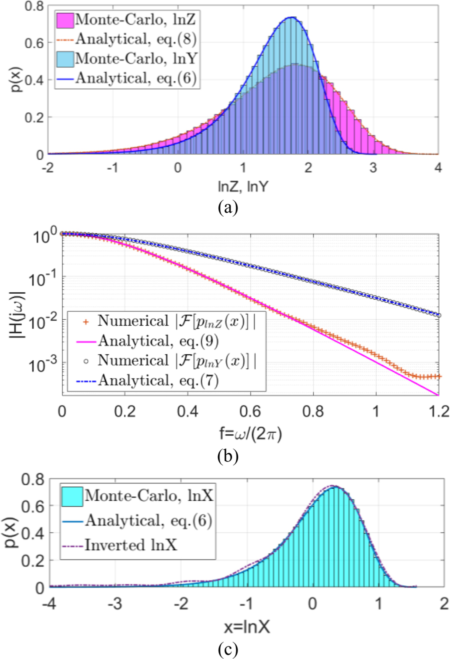
Figure 2: (a) The PDF plots of $\ln Z$ and $\ln Y$, (b) the magnitude of the Fourier transforms, and (c) the inverted PDF of $\ln X$ and analytical expression.

Instead of using the magnitude of the E-field, the derivations can also be verified using the received power. Suppose

$$p_{{\mathrm{x}}^2}\left(x\right)=e^{-\frac{x}{u_x}}/u_x,x=P_x,$$

(10)

where the expected value and the standard deviations are both $u_x$ ($u_x=2{\sigma }_x^2$). The power transfer function $Y^2$ has a PDF similar with (10). The PDF of the output power $Z^2=X^2\times Y^2$ can be obtained as

$$p_{Z^2}\left(z\right)=\frac{2}{u_x{u}_y}{K}_0\left(2\sqrt{\frac{z}{u_x{u}_y}}\right),z=P_{\mathrm{out}},$$

(11)

where $u_y=2{\sigma }_y^2$ is the expected value of $p_{{\mathrm{Y}}^2}\left(y\right)$. The expected value and the standard deviation of (11) can be derived as $u_x{u}_y$ and $u_x{u}_y\sqrt{3}$ respectively.

Measurement verifications were performed in an RC with inner dimensions of 0.94 m $\times$ 1.16 m $\times$ 1.44 m. Two stirrers were rotated synchronously with 1${}^{\circ }$/step, and 360 stirrer positions were used. Twenty-one frequency samples were collected in the frequency range of 5.98 GHz – 6.02 GHz at each stirrer position. With 360 stirrer positions, we have 21$\times$360=7560 samples and the PDF of the magnitude of the measured $S_{21}$ is illustrated in Fig. 3 (a). By tuning the magnitude of the input signal at each frequency and each stirrer position,

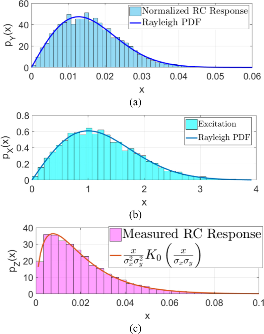
Figure 3: (a) PDF plot of the measured normalized E-field transfer function, (b) PDF plot of excited samples, and (c) PDF plot of the magnitude of the output E-field.

the output PDF can be shaped. Instead of using a constant input magnitude, ${\sigma }_x$ is used to control the mean value of the voltage, random voltage samples with a Rayleigh distribution of ${\sigma }_x=1$ V/m were generated to excite the RC as shown in Fig. 3 (b). The output histogram and the analytical equation plot are illustrated in Fig. 3 (c). Not surprisingly, a double-Rayleigh PDF was obtained for the RC response which agrees well with the analytical expression.

IV. LIMITATIONS AND GENERALIZATIONS

We have demonstrated that the PDF of the output of an RC can be synthesized with controlled input. This technique could be applied to scenarios involving channel emulations in multi-cavities. However, the output PDF cannot be arbitrary. Intuitively, one cannot synthesize a constant output (the PDF is $\delta \left(x-x_0\right)$) to eliminate the inherent statistical property of an RC. It has been shown that the Fourier transform $H_X\left(j\omega \right)$ of a PDF $p_X\left(x\right)$ (also named as characteristic function with $j$ replaced by $--j$) has some characteristics [14]:

1) $H_X\left(0\right)=1$, it is non-vanishing in a region around zero;

2) $\left|H_X\left(j\omega \right)\right|\le 1$, it is bounded;

3) $H_X\left(-j\omega \right)=H_X{\left(j\omega \right)}^{*}$, it is Hermitian.

Thus when two random variables are multiplied, we have$\left|H_X\left(j\omega \right)\right|\left|H_Y\left(j\omega \right)\right|\le \left|H_Y\left(j\omega \right)\right|$ and it is impossible to generate $\left|H_Z\left(j\omega \right)\right|>\left|H_Y\left(j\omega \right)\right|$. The inequality for the relative standard deviations can be derived as ${\mathrm{std}}_{\mathrm{rel}}\left(Z\right)={\mathrm{std}}_{\mathrm{rel}}(X\times Y)\ge {\mathrm{std}}_{\mathrm{rel}}(Y)$. The proof is detailed as follows:

From the mean inequality we have $\sqrt{\frac{1}{n}{\sum }_{i=1}^n{x}_i^2}\ge \frac{1}{n}{\sum }_{i=1}^n{x}_i$, thus the integral form is $\sqrt{{\int }_{-\mathrm{\infty }}^{+\mathrm{\infty }}{p}_X\left(x\right)x^{2}dx}\ge {\int }_{-\mathrm{\infty }}^{+\mathrm{\infty }}{p}_X\left(x\right)xdx$. When $X$ and $Y$ are positive random variables (e.g., E-field magnitude, power):

$${\int }_0^{\mathrm{\infty }}{p}_X\left(x\right)x^2\mathit{d}x\ge {\left({\int }_0^{\mathrm{\infty }}{p}_X\left(x\right)x\mathit{d}x\right)}^2,$$

(12)

${\displaystyle {\int }_0^{\mathrm{\infty }}}{p}_X\left(x\right)x^{2}dx{\displaystyle {\int }_0^{\mathrm{\infty }}}{p}_Y\left(x\right)x^{2}dx-{\left({\displaystyle {\int }_0^{\mathrm{\infty }}}{p}_X\left(x\right)xdx{\displaystyle {\int }_0^{\mathrm{\infty }}}{p}_Y\left(x\right)xdx\right)}^2$
$\ge {\left({\displaystyle {\int }_0^{\mathrm{\infty }}}{p}_X\left(x\right)xdx\right)}^2\left[{\displaystyle {\int }_0^{\mathrm{\infty }}}{p}_Y\left(x\right)x^{2}dx-{\left({\displaystyle {\int }_0^{\mathrm{\infty }}}{p}_Y\left(x\right)xdx\right)}^2\right],$	(13)

$$\frac{\sqrt{{\int }_0^{\mathrm{\infty }}{p}_X\left(x\right)x^{2}dx{\int }_0^{\mathrm{\infty }}{p}_Y\left(x\right)x^{2}dx-{\left({\int }_0^{\mathrm{\infty }}{p}_X\left(x\right)xdx{\int }_0^{\mathrm{\infty }}{p}_Y\left(x\right)xdx\right)}^2}}{{\int }_0^{\mathrm{\infty }}{p}_X\left(x\right)xdx{\int }_0^{\mathrm{\infty }}{p}_Y\left(x\right)xdx}$$

$$\ge \frac{\sqrt{{\int }_0^{\mathrm{\infty }}{p}_Y\left(x\right)x^{2}dx-{\left({\int }_0^{\mathrm{\infty }}{p}_Y\left(x\right)xdx\right)}^2}}{{\int }_0^{\mathrm{\infty }}{p}_Y\left(x\right)xdx},$$

(14)

which is ${\mathrm{std}}_{\mathrm{rel}}(X\times Y)\ge {\mathrm{std}}_{\mathrm{rel}}(Y)$. This means that the relative standard deviation of the output cannot be reduced when the input is also a random variable.

The results can be generalized to multiple cascading cavities as shown in Fig. 1 (b). When the couplings between cavities are small and the transfer functions are independent, the output can be expressed in the form of $Y={\prod }_{i=1}^n{Y}_i$. If each $Y_i$ has a Rayleigh distribution with parameter ${\sigma }_i$, the PDF of $Y$ can be derived as

$$p_{\mathrm{\Pi }}\left(y\right)=2^{\frac{n^2-4n+2}{2}}{y}^{3-n}{\sigma }_{\mathrm{\Pi }}^{n-4}\times$$

$$G([[],[]],[[a_1,a_2,\mathrm{\dots },a_n],[]],\frac{y^2}{2^n{\sigma }_{\mathrm{\Pi }}^2}),$$

(15)

where $G(\bullet )$ is the Meijer G-function defined in [15], $a_1=a_2=\mathrm{\cdots }=a_n=\left(n-2\right)/2$ and ${\sigma }_{\mathrm{\Pi }}={\prod }_{i=1}^n{\sigma }_i$. The expected value and the standard deviations are ${\left(\pi /2\right)}^{n/2}{\sigma }_{\mathrm{\Pi }}$ and $2^{-n/2}{\sigma }_{\mathrm{\Pi }}\sqrt{4^n-{\pi }^n}$ respectively. When $n\to \mathrm{\infty }$, the relative standard deviation approximates to

$$\underset{n\to \mathrm{\infty }}{lim}\frac{2^{-n/2}{\sigma }_{\mathrm{\Pi }}\sqrt{4^n-{\pi }^n}}{{\left(\pi /2\right)}^{n/2}{\sigma }_{\mathrm{\Pi }}}=\underset{n\to \mathrm{\infty }}{lim}\frac{2^{-n/2}\sqrt{4^n-{\pi }^n}}{{\left(\pi /2\right)}^{n/2}}\sim {\left(\frac{2}{\sqrt{\pi }}\right)}^n.$$

(16)

It is interesting to note that the relative standard deviation does not depend on parameters ${\sigma }_1,{\sigma }_2,\mathrm{\dots },{\sigma }_n$ and is only a function of cavity number $n$. Similarly, when each $Y_i^2$ has an exponential distribution with parameter $u_i$, the PDF of the power transfer function $Y^2={\prod }_{i=1}^n{Y}_i^2$ can be obtained as

$$p_{{\mathrm{\Pi }}^2}\left(y\right)=y^{2-n}{u}_{\mathrm{\Pi }}^{n-3}\times$$

$$G([[],[]],[[b_1,b_2,\mathrm{\dots },b_n],[]],\frac{y}{u_{\mathrm{\Pi }}}),$$

(17)

where $b_1=b_2=\mathrm{\cdots }=b_n=n-2$ and $u_{\mathrm{\Pi }}={\prod }_{i=1}^n{u}_i$. The expected value and the standard deviations are $u_{\mathrm{\Pi }}$ and $u_{\mathrm{\Pi }}\sqrt{2^n-1}$ respectively. Approximately, when $n$ is large, by applying the CLT (Central Limit Theorem), $\ln Y={\sum }_{i=1}^n\ln Y_i$. $\ln Y$ can be approximated using a normal distribution $N(\mu ,\sigma )$. It can be found that $\mu =n\left(\mathrm{ln2}-\gamma \right)/2+\ln {\sigma }_{\mathrm{\Pi }}$ and $\sigma =\pi \sqrt{6n}/12$. By applying the variable transform $e^Y$ to $\ln Y$, a lognormal PDF for $Y$ can be obtained which is [16]

$$p\left(y\right)={\text{e}}^{-\frac{{(\mu -\ln y)}^2}{2{\sigma }^2}}/\left(y\sigma \sqrt{2\pi }\right),$$

(18)

where the mean value and the standard deviations are ${\text{e}}^{\mu +{\sigma }^2/2}$ and $\sqrt{{\text{e}}^{2\mu +{\sigma }^2}({\text{e}}^{{\sigma }^2}-1)}$, respectively. It is interesting to note that, although the PDF can be well approximated for $\ln Y$ by using the CLT, because of the exponential function, the mean value from the lognormal PDF is biased, i.e. ${\text{e}}^{\mu +{\sigma }^2/2}\ne {\left(\pi /2\right)}^{n/2}{\sigma }_{\mathrm{\Pi }}$.

Note that we have not considered the time domain (TD) response in this work. To shape the power delay profile of the output, we may need to shape the input signal in the TD. This has been achieved by using a channel emulator in [11]. It is also possible to use a single signal generator to achieve similar results, however, to shape the output statistics in both FD and TD is still challenging. We only emulate FD responses in this paper, when the statistical properties of the FD and TD response of a system are both in constraints, TD operations (deconvolutions with the impulse responses) would be necessary. To emulate this scenario, it would be necessary to use the measured impulse responses from multi-cavities and control the excited impulse signals precisely in the TD if a single cavity is used.

ACKNOWLEDGMENT

This work was supported in part by the National Defense Basic Scientific Research Program of China under Grant JCKYS2021DC05, the Fund of Prospective Layout of Scientific Research for NUAA (Nanjing University of Aeronautics and Astronautics) and the Fundamental Research Funds for the Central Universities, Grant Number: NS2021029.

REFERENCES

[1] Electromagnetic Compatibility (EMC) – Part 4-21: Testing and Measurement Techniques – Reverberation Chamber Test Methods, IEC 61000-4-21, Ed 2.0, 2011.

[2] CTIA, Test Plan for Wireless Large-Form-Factor Device Over-the-Air Performance, ver. 1.2.1, Feb. 2019.

[3] D. A. Hill, Electromagnetic Fields in Cavities: Deterministic and Statistical Theories, Wiley-IEEE Press, Hoboken, NJ, 2009.

[4] C. L. Holloway, D. A. Hill, J. M. Ladbury, P. F. Wilson, G. Koepke, and J. Coder, “On the use of reverberation chambers to simulate a Rician radio environment for the testing of wireless devices,” IEEE Transactions on Antennas and Propagation, vol. 54, no. 11, pp. 3167-3177, Nov. 2006.

[5] E. Genender, C. L. Holloway, K. A. Remley, J. M. Ladbury, G. Koepke, and H. Garbe, “Simulating the multipath channel with a reverberation chamber: application to bit error rate measurements,” IEEE Transactions on Electromagnetic Compatibility, vol. 52, no. 4, pp. 766-777, Nov. 2010.

[6] J. D. Sanchez-Heredia, J. F. Valenzuela-Valdes, A. M. Martinez-Gonzalez, and D. A. Sanchez-Hernandez, “Emulation of MIMO Rician-Fading environments with mode-stirred reverberation chambers,” IEEE Transactions on Antennas and Propagation, vol. 59, no. 2, pp. 654-660, Feb. 2011.

[7] J. Frolik, T. M. Weller, S. DiStasi, and J. Cooper, “A compact reverberation chamber for hyper-Rayleigh channel emulation,” IEEE Transactions on Antennas and Propagation, vol. 57, no. 12, pp. 3962-3968, Dec. 2009.

[8] J. D. Sánchez-Heredia, M. A. García-Fernández, M. Grudén, P. Hallbjörner, A. Rydberg, and D. A. Sánchez-Hernández, “Arbitrary fading emulation using mode-stirred reverberation chambers with stochastic sample handling,” Proceedings of the 5th European Conference on Antennas and Propagation (EUCAP), pp. 152-154,2011.

[9] C. Wright and S. Basuki, “Utilizing a channel emulator with a reverberation chamber to create the optimal MIMO OTA test methodology,” Global Mobile Congress, pp. 1-5, 2010.

[10] J. Kvarnstrand, E. Silfverswärd, D. Skousen, D. Reed, and A. Rodriguez-Herrera, “Mitigation of double-Rayleigh fading when using reverberation chamber cascaded with channel emulator,” 12th European Conference on Antennas and Propagation (EuCAP 2018), London, UK, pp. 1-5, Apr. 2018.

[11] H. Fielitz, K. A. Remley, C. L. Holloway, Q. Zhang, Q. Wu, and D. W. Matolak, “Reverberation-chamber test environment for outdoor urban wireless propagation studies,” IEEE Antennas and Wireless Propagation Letters, vol. 9, pp. 52-56, Feb. 2010.

[12] Q. Xu, L. Xing, Y. Zhao, T. Jia, and Y. Huang, “Probability distributions of three-antenna efficiency measurement in a reverberation chamber,” IET Microwaves, Antennas & Propagation, vol. 15, no. 12, pp. 1545-1552, May 2021.

[13] M. Höijer and L. Kroon, “Field statistics in nested reverberation chambers,” IEEE Transactions on Electromagnetic Compatibility, vol. 55, no. 6, pp. 1328-1330, Dec. 2013.

[14] F. Oberhettinger, Fourier Transforms of Distributions and their Inverses, Academic Press, New York, 1973.

[15] F. W. J. Oliver, D. W. Lozier, R. F. Boisvert, and C. W. Clark, NIST Handbook of Mathematical Functions, Cambridge University Press, Cambridge, UK, 2010.

[16] G. Gradoni, J.-H. Yeh, B. Xiao, T. M. Antonsen, S. M. Anlage, and E. Ott, “Predicting the statistics of wave transport through chaotic cavities by the random coupling model: A review and recent progress,” Wave Motion, vol. 51, pp. 606-621, June 2014.

BIOGRAPHIES

Qian Xu (Member, IEEE) received the B.Eng. and M.Eng. degrees from the Department of Electronics and Information, Northwestern Polytechnical University, Xi’an, China, in 2007 and 2010, and received the PhD degree in Electrical Engineering from the University of Liverpool, UK, in 2016. He is currently an Associate Professor at the College of Electronic and Information Engineering, Nanjing University of Aeronautics and Astronautics, China.

He was as a RF engineer in Nanjing, China in 2011, an Application Engineer at CST Company, Shanghai, China in 2012. His work at University of Liverpool was sponsored by Rainford EMC Systems Ltd. (now part of Microwave Vision Group) and Centre for Global Eco-Innovation. He has designed many chambers for the industry and has authored the book Anechoic and Reverberation Chambers: Theory, Design, and Measurements (Wiley-IEEE, 2019). His research interests include statistical electromagnetics, reverberation chamber, EMC, and over-the-air testing.

Feng Tian received the B.Eng. degree from University of Electronic Science and Technology of China, Chengdu, China, in 2008, and received M.Eng. degree from CETC 14th Institute, Nanjing, China, in 2011. He is currently a PhD student at the College of Electronic and Information Engineering, Nanjing University of Aeronautics and Astronautics, China. His research interests include power amplifier, EMC, and antennas.

Yongjiu Zhao received the M.Eng. and Ph.D. degrees in Electronic Engineering from Xidian University, Xi’an, China, in 1990 and 1998, respectively. Since March 1990, he has been with the Department of Mechano-Electronic Engineering, Xidian University where he was a professor in 2004. From December 1999 to August 2000, he was a Research Associate with the Department of Electronic Engineering, The Chinese University of Hong Kong. His research interests include antenna design, microwave filter design and electromagnetic theory.

Rui Jia received the B.Eng. degrees from the Department of Electronics and Information, Zhengzhou University, Zhengzhou, China, in 2008, and received the M.Eng. and Ph.D. degrees in Electronic Engineering from Mechanical Engineering College, Shijiazhuang, China, in 2010 and 2014, respectively. His research interests include statistical electromagnetics, reverberation chamber, and EMC.

Erwei Cheng nreceived the M.Eng. degrees in Electronic Engineering from Mechanical Engineering College, Shijiazhuang, China, in 2009. He is currently an Associate Professor at the National Key Laboratory on Electromagnetic Environment Effects, Army Engineering University Shijiazhuang Campus, China.

Lei Xing received the B.Eng. and M.Eng. degrees from the School of Electronics and Information, Northwestern Polytechnical University, Xi’an, China, in 2009 and 2012. She received PhD degree in Electrical Engineering and Electronics at the University of Liverpool, UK, in 2015. She is currently an Associate Professor at the College of Electronic and Information Engineering, Nanjing University of Aeronautics and Astronautics, China.

ACES JOURNAL, Vol. 38, No. 4, 263–268
doi: 10.13052/2023.ACES.J.380405
© 2023 River Publishers

ABSTRACT

I. INTRODUCTION

II. THEORY

III. DERIVATIONS AND VERIFICATIONS

IV. LIMITATIONS AND GENERALIZATIONS

ACKNOWLEDGMENT

REFERENCES

BIOGRAPHIES