Wideband Monostatic RCS Prediction of Complex Objects using Support Vector Regression and Grey-wolf Optimizer

Zhourui Zhang${}^{\mathbf{\text{1}}}$, Pengyuan Wang${}^{\mathbf{\text{2}}}$, and Mang He${}^{\mathbf{\text{3}}}$

¹School of Integrated Circuits and Electronics
Beijing Institute of Technology, Beijing, 100081, China
3120215371@bit.edu.cn
²School of Integrated Circuits and Electronics
Beijing Institute of Technology, Beijing, 100081, China
3120205355@bit.edu.cn
³School of Integrated Circuits and Electronics
Beijing Institute of Technology, Beijing, 100081, China
hemang@bit.edu.cn

Submitted On: February 21, 2023; Accepted On: September 29, 2023

ABSTRACT

This paper presents a method based on the support vector regression (SVR) model and grey wolf optimizer (GWO) algorithm to efficiently predict the monostatic radar cross-section (mono-RCS) of complex objects over a wide angular range and frequency band. Using only a small-size of the mono-RCS data as the training set to construct the SVR model, the proposed method can predict accurate mono-RCS of complex objects under arbitrary incident angle over the entire three-dimensional space. In addition, the wideband prediction capability of the method is significantly enhanced by incorporating the meta-heuristic algorithm GWO. Numerical experiments verify the efficiency and accuracy of the proposed SVR-GWO model over a wide frequency band.

Index Terms: Complex objects, grey wolf optimizer, machine learning, radar cross-section, support vector regression.

I. INTRODUCTION

Radar cross-section (RCS) is one of the most important concepts in radar stealth technology [1], and the traditional methods for RCS estimation can be divided into two categories. One type is the full-wave numerical method, which has high accuracy but is time-consuming and computationally expensive. The other one is the high-frequency approximate method, which is fast but precision-limited. A common shortage of these methods is the incapability to accomplish the RCS of radar targets in real-time, especially for the monostatic RCS (mono-RCS) prediction of complex objects because it usually takes long computation time for each incident angle repeatedly. Therefore, new approaches are required to address the problem of real-time mono-RCS computation.

Due to the regression capability of nonlinear fitting and generalization ability, machine learning (ML) has recently been applied in solving computational electromagnetics (EM) problems. An essential benefit of ML is that once the relationship has been established between the input and output spaces, the results for any other given inputs can be predicted instantaneously, which could save computation resources massively. Researchers have proposed ML models for EM solver design [2], repairing damaged receivers’ data [3], and low scattering meta-surface design [4], etc. ML has also been applied in RCS prediction [5–10], but the existing techniques still have some limitations. For instance, 8326 samples are required for a single frequency point in [5], which may not be applicable for computationally expensive EM problems. The ML models in [6, 7] are effective only when the direction of the incident wave varies in one direction ($\theta$ or $\phi$ direction), which ignore the mono-RCS variation in the entire space. The physics-inspired model in [9] is suitable for the mono-RCS estimation at a single frequency point, while its wideband performance is not further considered. [10] discusses the RCS prediction over a wide frequency band, but the aspect angle variation range is only 10 degrees, and the sampling interval is very close (0.2-degree step), which results in massive computational costs. To the best of our knowledge, few works have been found to solve the problem of fast and accurate mono-RCS prediction in real-time using ML over a wide range of incident angles and wide frequency bands simultaneously.

This work proposes an alternative method that combines the support vector regression (SVR) model and grey-wolf optimizer (GWO) [11] to predict the mono-RCS of complex targets under any incident angle over a wide frequency band. The proposed method employs the SVR model to establish the approximate function between mono-RCS and incident angle and frequency, i.e., RCS ($\theta$, $\phi$, f). The metaheuristic algorithm GWO is applied to accomplish the parameter optimization of the SVR model and achieves better prediction ability in comparison with other metaheuristic algorithms. Unlike the existing deep learning (DL) algorithms that need enormous datasets, the new SVR-GWO model achieves high-accuracy prediction and has robust generalization to unknown samples by using small-sized training datasets, which is crucial for mono-RCS prediction of complex targets that need extensive computation. With a well-trained SVR- GWO model, for arbitrary angle of incidence, the mono-RCS of complex targets over a wide frequency band can be predicted with good accuracy almost in real time.

II. SVR-GWO METHOD

In order to achieve fast prediction of wideband mono-RCS of complex targets under the arbitrary incident angle, the SVR model representing the nonlinear relationship between the mono-RCS and input parameters, i.e., the operating frequency f and the angle of incidence ($\theta$, $\phi$), should be first constructed. Typical mono-RCS data need to be sampled within the target frequency band and angular range, and the approximation function of the mono-RCS and input parameters can be represented [12] as:

$$f\left({\mathbf{x}}_{\mathbf{i}}\right)={\mathbf{w}}^T\varphi \left({\mathbf{x}}_{\mathbf{i}}\right)+b,$$

(1)

where $\varphi ({\mathbf{x}}_{\mathbf{i}})$ is the nonlinear function of the input parameter vector ${\mathbf{x}}_{\mathbf{i}}$ that consists of f, $\theta$, and $\phi$, and $f({\mathbf{x}}_{\mathbf{i}})$ is the output of the SVR model; i.e. the predicted value of mono-RCS for the target. ${\mathbf{w}}^T$ and $b$ are weight and bias vectors, respectively.

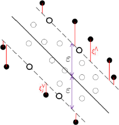
Figure 1: Diagram of the SVR model.

As shown in Fig. 1, the SVR model assumes that a deviation of at most $\epsilon$ between the predicted value of the mono-RCS and its true value (obtained from accurate numerical calculations) can be tolerated, which is called the $\epsilon$-tube. The slack variable $\xi$ is often introduced to measure the deviation of data points beyond the $\epsilon$-tube, representing a soft margin that the SVR model allows some samples not to satisfy the constraints [13]. Thus, the SVR model aims to optimize the following constrained target function [12]:

	$\underset{\mathbf{w},b}{min}{\displaystyle \frac{1}{2}}{\parallel \mathbf{w}\parallel }_2^2+C{\displaystyle \sum _{i=1}^n}({\xi }_i^{\vee }+{\xi }_i^{\wedge }),$
	$\mathrm{s}.\mathrm{t}.\mathit{\hspace{1em}}-\epsilon -{\xi }_i^{\vee }\le |y_i-({\mathbf{w}}^T\varphi \left(x_i\right)+b)|\le \epsilon +{\xi }_i^{\wedge },$
	${\xi }_i^{\bigvee }\ge 0,{\xi }_i^{\bigwedge }\ge 0,i=1,2,3\mathrm{\dots }n,$		(2)

where $y_i$ is the true value of mono-RCS, and $C$ is a constant called the penalty parameter. When $C$ is infinitely large, equation (2) forces all samples to fulfill constraints but tends to cause the model overfitting. If $C$ has a finite value, the model allows some samples not to fall into the $\epsilon$-tube, and the variables ${\xi }_i^{\vee }$ and ${\xi }_i^{\wedge }$ determine the allowable deviation below and above the $\epsilon$-tube, respectively.

The constrained optimization problem can be reformulated into a pairwise problem form using the Lagrangian multiplier approach. By doing so, the correlation of the input and output of the SVR model [12] becomes:

$$f({\mathbf{x}}_{\mathbf{i}})=\sum _{i=1}^N({\alpha }_i,{\alpha }_i^{*})K(x,x_i)+b,$$

(3)

where ${\alpha }_i$ and ${\alpha }_i^{*}$ are the Lagrangian multipliers. $K(x,x_i)$ is the kernel function, representing the inner product of $x_i$ and $x_j$ in their feature space $\varphi (x_i)$ and $\varphi (x_j)$.

In this paper, the radial basis function (RBF) [12] is chosen as the kernel function due to its capability for nonlinear fitting and relatively fewer parameters:

$$K(x_i,x_j)=exp\left(-\gamma {\parallel x_i-x_j\parallel }^2\right).$$

(4)

Once the SVR model is constructed, its accuracy should be verified by the validation set. The coefficient of determination $R^2$ defined in [14] is applied to measure the goodness of the SVR model:

$$R^2=1-\frac{{\sum }_i{\left(y_i-{\widehat{y}}_i\right)}^2}{{\sum }_i{\left(y_i-\overline{y}\right)}^2},$$

(5)

where ${\widehat{y}}_i$ is the predicted mono-RCS, and $\overline{y}$ is the mean of the true value of mono-RCS $y_i$. Apparently, the range of $R^2$is [0, 1], and the higher the value is, the better the model fits.

As mentioned before, the penalty parameter C and threshold tolerance $\epsilon$ are crucial for constructing a high-precision SVR model and must be pre-determined before applying the Lagrangian multiplier approach. Similarly, the parameter $\gamma$ in the kernel RBF should also be pre-determined. In this paper, the recently proposed GWO algorithm [11] is utilized to optimize the parameters of the SVR model for better performance, and the optimal solution of the target function $R^2$ is obtained by parameter search within the range of values of the input parameters C, $\epsilon$, and $\gamma$.

The GWO algorithm mimics the leadership hierarchy and hunting mechanism of grey wolves in nature. A wolf pack is created and is used to search for the optimal solution. In the first iteration, each individual’s position, i.e., the values of input parameters, are randomly allocated, and the corresponding $R^2$ is calculated and ranked. Wolf $\alpha$, $\beta$, $\delta$ are assumed to learn better about the position of the optimal solution and keep the best three solutions for the current iteration. Other individuals search for the position of the better solution based on the positions of the best three solutions [11] by

$$\{\begin{array}{c}\hfill \stackrel{\rightharpoonup }{\mathit{D}}=|\stackrel{\rightharpoonup }{\mathit{C}}\cdot \stackrel{\rightharpoonup }{\mathit{X}}-\stackrel{\rightharpoonup }{\mathit{X}}(t)|\hfill \\ \hfill \stackrel{\rightharpoonup }{\mathit{D}}=|\stackrel{\rightharpoonup }{\mathit{C}}\cdot \stackrel{\rightharpoonup }{\mathit{X}}-\stackrel{\rightharpoonup }{\mathit{X}}(t)|\hfill \\ \hfill \stackrel{\rightharpoonup }{\mathit{D}}=|\stackrel{\rightharpoonup }{\mathit{C}}\cdot \stackrel{\rightharpoonup }{\mathit{X}}-\stackrel{\rightharpoonup }{\mathit{X}}(t)|\hfill \end{array},$$

(6)

$$\{\begin{array}{c}\hfill \stackrel{\rightharpoonup }{\mathit{X}}=\stackrel{\rightharpoonup }{\mathit{X}}-\stackrel{\rightharpoonup }{\mathit{A}}\cdot \stackrel{\rightharpoonup }{\mathit{D}}\hfill \\ \hfill \stackrel{\rightharpoonup }{\mathit{X}}=\stackrel{\rightharpoonup }{\mathit{X}}-\stackrel{\rightharpoonup }{\mathit{A}}\cdot \stackrel{\rightharpoonup }{\mathit{D}}\hfill \\ \hfill \stackrel{\rightharpoonup }{\mathit{X}}=\stackrel{\rightharpoonup }{\mathit{X}}-\stackrel{\rightharpoonup }{\mathit{A}}\cdot \stackrel{\rightharpoonup }{\mathit{D}}\hfill \end{array},$$

(7)

$$\stackrel{\rightharpoonup }{\mathit{X}}\left(t+1\right)=\frac{\stackrel{\rightharpoonup }{\mathit{X}}+\stackrel{\rightharpoonup }{\mathit{X}}+\stackrel{\rightharpoonup }{\mathit{X}}}{3},$$

(8)

where $t$ means the iteration number, and $\stackrel{\rightharpoonup }{\mathit{A}}$ and $\stackrel{\rightharpoonup }{\mathit{C}}$ (= 1, 2, 3) are the vectors of coefficients. $\stackrel{\rightharpoonup }{\mathit{A}}$ is a random vector with its entry being in the range of [-2,+2] and gradually shrinks toward 0 with iterations. When $\left|\stackrel{\rightharpoonup }{\mathit{A}}\right|<1,$the individual approaches the target position; otherwise, the individual is forced to search for the more suitable position. $\stackrel{\rightharpoonup }{\mathit{C}}$ is a random vector with its entry being between 0 and 2, and $\stackrel{\rightharpoonup }{\mathit{X}}$ is each individual’s position vector, representing the values of input parameters. $\stackrel{\rightharpoonup }{\mathit{X}}(k=\alpha ,\beta ,\delta )$ denotes the position of the best three solutions, and $\stackrel{\rightharpoonup }{\mathit{D}}$ means the distance between the individual’s position and the position of the best three solutions. The search and individual sorting are repeated until the error is satisfied or the maximum number of iteration steps is reached. The final position of the wolf $\alpha$, which is the optimal solution of the input parameters in their domain, is returned.

The flowchart of the proposed SVR-GWO method is shown in Fig. 2. It starts from the construction of the SVR model, then hyperparameters of the SVR model are tuned by the GWO algorithm. By evaluating the coefficient of determination for each individual, optimal hypermeters are selected to update the SVR model until reaching the final convergence.

III. NUMERICAL VALIDATION

In this section, the predicted mono-RCS of complex targets by the SVR-GWO method are compared with the true values from full-wave numerical calculations to evaluate the accuracy and effectiveness of the proposed model. The sampling datasets are achieved by an in-house multilevel fast multipole algorithm (MLFMA) accelerated volume-surface integral equation (VSIE) solver (referred to as the VSIE-MLFMA hereinafter) [15], and the computing platform is a personal computer with an Intel i5-10400 2.9 GHz CPU and 16 GB RAM. The proposed method is implemented in PyCharm.

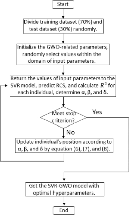
Figure 2: Flowchart of the SVR-GWO method.

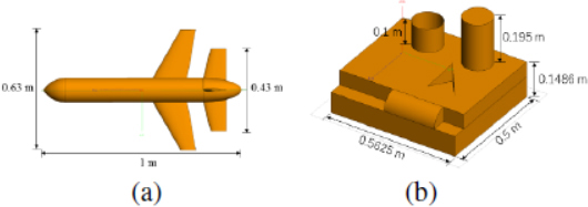
Figure 3: The geometries of two numerical models: (a) missile and (b) SLICY.

A. Mono-RCS of a missile model

The geometry of the perfect electric conductor (PEC) missile model is shown in Fig. 3 (a), and it is illuminated by a vertically polarized plane wave with a frequency varying from 0.3 to 0.7 GHz. The predicted mono-RCS of the missile model at 0.6 GHz is first used to demonstrate the accuracy of the SVR-GWO method for single frequency point. Figure 4 shows good agreement between predicted values and true values in a wide angular range. The wideband performance of the proposed method is verified in Fig. 5, in which the comparison of the mono-RCS between predicted values and true values is shown at four different frequencies (0.325, 0.425, 0.575, and 0.675 GHz). For the training and testing datasets of the model, the sampling interval of incident angle in both $\theta$ and $\phi$ directions is 3°, with $\theta$ varying from 0°to 90°, and $\phi$ varying from 0°to 360°in the single frequency case and from 0° to 180° in the wideband case; the sampling interval of frequency is 0.05 GHz. In all cases, 70% of sampling data are used for training, and 30% are used for testing. Therefore, the sizes of sampling datasets are 3751 in the single frequency case and 17,019 in the broadband prediction, respectively.

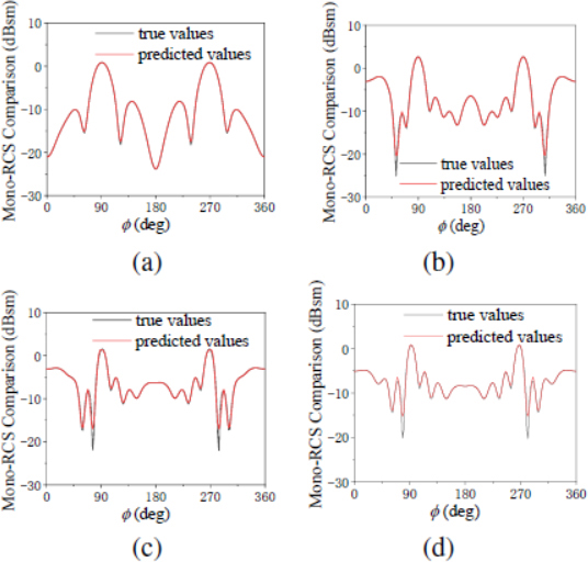
Figure 4: Comparison of the predicted mono-RCS with the true values at 0.6 GHz for fixed elevation angles (a) $\theta$ = 30°, (b) $\theta$ = 50°, (c) $\theta$ = 70°, and (d) $\theta$ = 80°.

Figure 5: Comparison of the predicted mono-RCS of the missile model and the true values under different incident angles at various frequencies: (a) $\theta$ = 75°, f = 0.325 GHz, (b) $\theta$ = 60°, f = 0.425 GHz, (c) $\theta$ = 48°, f = 0.575 GHz, and (d) $\theta$ = 36°, f = 0.675 GHz.

The root mean square error (RMSE) [16] is used to evaluate the prediction performance of the SVR-GWO model, which is defined as:

$$RMSE=\sqrt{\frac{1}{n}\sum _{i=1}^n{({\widehat{y}}_i-y_i)}^2}.$$

(9)

Table 1: Comparison of RMSE and cost time with different models

Models	RMSE (dBsm)	Cost Time (s)
Proposed method	1.48	21,711
SVR-PSO	2.17	89,568
SVR	3.99	N/A
BP neural network	2.51	51,84
GPR	1.71	13,053
PCE	3.41	1,673
LRA	5.10	476

The RMSE and the cost time of the missile model were also calculated using following methods: The SVR model optimized by particle swarm optimizer (PSO); the SVR model without any optimizer; the backward propagation (BP) neural network [5–7]; the Gaussian process regression (GPR) model [8]; the polynomial chaos expansion (PCE) [17], and the low rank approximation (LRA) [18].

The comparison of different models is given in Table 1. The results prove the prediction accuracy and the efficacy of the proposed method. The RMSE of the SVR-GWO model is 62.9% and 31.8% lower than those of the SVR and the SVR-PSO models, respectively, and the training time is reduced by 75.8%. Compared with algorithms in similar literatures or other ML benchmark techniques, the RMSE of the missile model is also reduced from 13% to 71%.

To evaluate the regression performance of the SVR- GWO model, Figs. 6 and 7 (a) show the deviation of the predicted mono-RCS of the missile model from the accurate ones by the VSIE-MLFMA solver at a single frequency (0.6 GHz) and at four typical frequencies (0.325, 0.425, 0.575, and 0.675 GHz) within a wide frequency band. Two types of validation datasets of the same size (2024) are used in Fig. 6. One dataset is generated by using uniform sampling, and the other one is obtained from random sampling. The RMSEs of the uniform and random samplings are 0.65 and 0.92 dBsm, respectively, while the training time used in both sampling schemes is almost the same (900 seconds). The results clearly indicate that the uniform sampling scheme is better for the proposed model. Numerical simulations also show that once the SVR-GWO model is well trained, it can predict the mono-RCS of over 2000 samples per second, which means nearly real-time RCS calculationcapability.

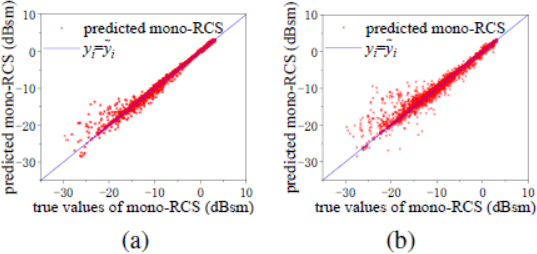
Figure 6: Deviation of the predicted values from the accurate mono-RCS of the missile at a single frequency: (a) Uniform sampling and (b) random sampling.

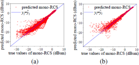
Figure 7: Deviation of the predicted values from the accurate mono-RCS of complex targets within a wide frequency band: (a) Missile model and (b) SLICY model.

B. Mono-RCS of the SLICY model

The geometry of the second example (a PEC SLICY [19] model), is shown in Fig. 3 (b), and a vertically polarized plane wave illuminates the target with the frequency varying from 0.6 to 1.4 GHz. To obtain the dataset used for training and testing, the sampling interval of frequency is 0.1 GHz. At each sampling frequency, the incident angles in both $\theta$ and $\phi$ directions vary from 0°to 90°with a 3°sampling interval. 70% of the samplings are used for training, and 30% are used for testing. Therefore, the size of the dataset is 8649.

Table 2: Comparison of RMSE and cost time with different models

Models	RMSE (dBsm)	Cost Time (s)
Proposed method	1.42	7,600
SVR-PSO	1.75	16,933
SVR	2.28	N/A
BP neural network	3.26	3,167
GPR	2.24	5,573
PCE	4.19	1,254
LRA	3.33	423

The mono-RCS values at four typical working frequencies (0.65, 0.75, 1.15, and 1.35 GHz) are selected for validation. For each frequency point, the incident angles $\theta$ and $\phi$ run from 0°to 90°, and the sampling interval in $\theta$ and $\phi$ directions are 3°and 1°, respectively. So the size of the validation dataset is 11,284. A comparison of the results between the RCS predicted by the SVR-GWO model and those calculated by the VSIE-MLFMA solver is shown in Fig. 8, and the predicted results are found in good agreement with the accurate values.

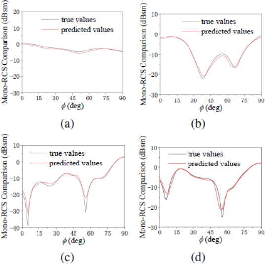
Figure 8: Comparison of the predicted mono-RCS of the SLICY model and the true values under different incident angles at various frequencies: (a) $\theta$ = 45°, f = 0.65 GHz, (b) $\theta$ = 51°, f = 0.95 GHz, (c) $\theta$ = 81°, f = 1.15 GHz, and (d) $\theta$ = 66°, f = 1.35 GHz.

Table 2 gives the RMSE and cost time comparison of different models. The RMSE of the SVR-GWO is 37.7% and 18.8% lower than those of the SVR and the SVR-PSO models, respectively, and the training time is reduced by 55.1%. It is seen that as the size of training data increases, the convergence speed of the GWO is faster compared to the PSO. Compared with algorithms in similar literatures or other ML benchmark techniques, the RMSE of the SLICY model is reduced from 36.6% to 66.1%. Figure 7 (b) illustrates the regression performance of the SVR- GWO model for the validation datasets of the SLICY model; again, the results indicate high prediction accuracy of the proposed method.

Table 3: RMSE and cost time comparison of proposed method with POI-SVR for SLICY model in 1 GHz

Model	RMSE (dBsm)	Cost Time (s)
SVR-GWO	0.59	373.8
POI-SVR	0.72	1240.5

In Table 3, the mono-RCS prediction capability of the proposed method for a single frequency point is compared with the physical-optics-inspired (POI) SVR [9], which is a physical-inspired method. As shown in the table, for mono-RCS prediction of target at a single frequency point, the proposed method achieves higher accuracy while reducing the training time compared to POI-SVR.

IV. CONCLUSION

In this paper, a method based on the SVR model and GWO algorithm is proposed to predict monostatic RCS with high accuracy and efficiency. Unlike the existing SVR models, the proposed SVR-GWO method can predict the monostatic RCS of complex targets simultaneously in a wide range of incident angles and within wide frequency bands. In addition, the new method needs relatively small training datasets and less training time, which is very important to realize real-time RCS prediction for computationally expensive complex targets.

ACKNOWLEDGEMENT

This project is supported by the Natural Science Foundation of China, No. 62171026.

REFERENCES

[1] D. K. Barton, Modern Radar System Analysis. Norwood, 1988.

[2] Z. Ma, K. Xu, R. Song, C. F. Wang, and X. Chen, “Learning-based fast electromagnetic scattering solver through generative adversarial network,” IEEE Trans. Antennas Propagat., vol. 69, no. 4, pp. 2194-2208, Apr. 2021.

[3] H. J. Hu, L. Y. Xiao, J. N. Yi, and Q. H. Liu, “Nonlinear electromagnetic inversion of damaged experimental data by a receiver approximation machine learning method,” IEEE Antennas Wireless Propagat. Lett., vol. 20, no. 7, pp. 1185-1189, July2021.

[4] S. Koziel and M. Abdullah, “Machine-learning-powered EM-based framework for efficient and reliable design of low scattering metasurfaces,” IEEE Trans. Microw. Theory Tech., vol. 69, no. 4, pp. 2028-2041, Apr. 2021.

[5] J. Guo, Y. Li, S. Cai, and D. Su, “Fast prediction of electromagnetic scattering characteristics of targets based on deep learning,” IEEE/ACES Int. Conf. Wireless Commun. Appl. Comput. Electromagn., pp. 1-2, 2021.

[6] P. Zhang, W. Liu, L. Guo, and J. She, “Efficient RCS prediction of composite scene based on deep BP neural networks,” 2021 Photonics & Electromagnetics Research Symposium (PIERS), pp. 1319-1325, 2021.

[7] Y. Zhao, J. Jiang, and L. Miao, “RCS prediction of polygonal metal plate based on machine learning,” IEEE/ACES Int. Conf. Wireless Commun. Appl. Comput. Electromagn., pp. 1-2, 2021.

[8] D. Xiao, L. Guo, W. Liu, and M. Hou, “Improved Gaussian process regression inspired by physical optics for the conducting target’s RCS prediction,” IEEE Antennas Wireless Propagat. Lett., vol. 19, no. 12, pp. 2403-2407, Dec. 2020.

[9] D. Xiao, L. Guo, W. Liu, and M. Hou, “Efficient RCS prediction of the conducting target based on physics-inspired machine learning and experimental design,” IEEE Trans. Antennas Propagat., vol. 69, no. 4, pp. 2274-2289, Apr. 2021.

[10] T. Yan, D. Li, and W. Yu, “A surrogate modeling technique based on space mapping for radar cross section,” IEEE Antennas Wireless Propagat. Lett., vol. 21, no. 8, pp. 1630-1633, Aug. 2022.

[11] S. Mirjalili, S. M. Mirjalili, and A. Lewis, “Grey wolf optimizer,” Adv. Eng. Softw., vol 69, pp. 46-61, Mar. 2014.

[12] S. R. Gunn, “Support vector machines for classification and regression,” ISIS Technical Report, vol. 14, no. 1, pp. 5-16, 1998.

[13] F. Pedregosa, G. Varoquaux, A. Gramfort, V. Michel, B. Thirion, O. Grisel, M. Blondel, P. Prettenhofer, R. Weiss, V. Dubourg, and J. Vanderplas, “Scikit-learn: machine learning in Python,” J. Mach. Learn. Res., vol. 12, pp. 2825-2830, 2011.

[14] D. Zhang, “A coefficient of determination for generalized linear models,” Am. Stat., vol. 71, no. 4, pp. 310-316, Oct. 2017.

[15] W. Q. Liu and M. He, “Accelerating solution of volume-surface integral equations with multiple right-hand sides by improved skeletonization techniques,” IEEE Antennas Wireless Propagat. Lett., vol. 18, no. 10, pp. 2006-2010, Oct. 2019.

[16] T. Chai and R. R. Draxler, “Root mean square error (RMSE) or mean absolute error (MAE)? - arguments against avoiding RMSE in the literature,” Geosci. Model Dev., vol. 7, no. 3, pp. 1247-1250, June 2014.

[17] G. J. K. Tomy and K. J. Vinoy, “A fast polynomial chaos expansion for uncertainty quantification in stochastic electromagnetic problems,” IEEE Antennas Wireless Propagat. Lett., vol. 18, no. 10, pp. 2120-2124, 2019.

[18] K. Konakli, C. Mylonas, S. Marelli, and B. Sudret, “Uqlab user manual-canonical low-rank approximations,” Report UQLab-V1, pp. 1-108, 2019.

[19] L. M. Yuan, Y. G. Xu, W. Ga, F. Dai, and Q. L. Wu, “Design of scale model of plate-shaped absorber in a wide frequency range,” Chin. Phys. B, vol. 27, no. 4, p. 044101, 2018.

BIOGRAPHIES

Zhourui Zhang received the B.S. degree in electrical engineering from Beijing Institute of Technology, Beijing, China, in July 2018, and the M.S. degree in electrical engineering from University of California, San Diego, US, in March 2021. He is currently pursuing the Ph.D. degree in electronic science and technology at the Beijing Institute of Technology, Beijing, China. His current research interest is yield and sensitivity analysis of antenna-radome systems.

Pengyuan Wang received the B.S. degree in communication engineering from North China Electric Power University, Baoding, China, in 2019. She is currently pursuing the Ph.D. degree in electromagnetics and microwave technology at the Beijing Institute of Technology, Beijing. Her current research interests include computational electromagnetics and parallel computation.

Mang He (Senior Member, IEEE) received the B.S. and Ph.D. degrees from the Department of Electrical Engineering, Beijing Institute of Technology, Beijing, China, in 1998 and 2003, respectively. From 2003 to 2004, he was a research associate with the Department of Electronic Engineering, City University of Hong Kong, Hong Kong. From 2008 to 2009, he was a post-doctoral research fellow with the Department of Electrical and Communication Engineering, Tohoku University, Sendai, Japan. He is currently a professor at the Beijing Institute of Technology. His current research interests include computational electromagnetics and its applications, antenna theory and design, radome, and frequency-selective surface design.

ACES JOURNAL, Vol. 38, No. 8, 609–615
doi: 10.13052/2023.ACES.J.380808
© 2023 River Publishers

ABSTRACT

I. INTRODUCTION

II. SVR-GWO METHOD

III. NUMERICAL VALIDATION

A. Mono-RCS of a missile model

B. Mono-RCS of the SLICY model

IV. CONCLUSION

ACKNOWLEDGEMENT

REFERENCES

BIOGRAPHIES