Antenna Shape Modeling based on Histogram of Oriented Gradients Feature
Hai-Ying Luo, Wen-Hao Su, Haiyan Ou, Sheng-Jun Zhang, and Wei Shao
1School of Physics
University of Electronic Science and Technology of China, Chengdu, 611731, China
hyluo@std.uestc.edu.cn, suwenhao1202@163.com, ouhaiyan@uestc.edu.cn, weishao@uestc.edu.cn
2National Key Laboratory of Science and Technology on Test Physics and Numerical Mathematics
Beijing 100076, China
zhangsj98@sina.com
Submitted On: February 27, 2023; Accepted On: May 1, 2023
ABSTRACT
A least square support vector machine (SVM) model is proposed for shape modeling of slot antennas. The slot image is mapped into the electromagnetic response by the SVM model. A modified shape-changing technique is also proposed to describe the antenna geometry by the quadratic uniform B-spline curve and generate the slot images. In the model, the histogram of oriented gradients feature is extracted from the slot images to show the appearance and shape of the slot. The relationship between the histogram of oriented gradient features and the electromagnetic responses is preliminarily built on SVM and the transfer function. Then a radial basis function network is used for error correction. The effectiveness of the proposed model is confirmed with an example of a tri-band microstrip-fed slot antenna. Compared with the convolutional neural network (CNN), the feature extracted by CNN is substituted by the histogram of oriented gradients feature, and the proposed model shows the same accuracy and the improvement of training efficiency.
Index Terms: B-spline curve, microstrip antenna, shape modeling, support vector machine.
I. INTRODUCTION
In recent years, the artificial neural network has been widely applied to the modeling of antennas, speeding up the design process [1–3]. The mapping relation between the antenna geometry and the electromagnetic response is learned by the neural network model. Although the generation of training and testing samples needs a certain number of full-wave simulations, the trained model can predict the response quickly and accurately.
A parametric model based on the artificial neural network is proposed for predicting the input resistance of a broadband antenna [4]. The frequency-dependent resistance envelope of the antenna is parametrized by a Gaussian model, and the neural network maps the geometrical parameter of the antenna to the Gaussian parameters. To build a neural network with high dimension of geometrical parameter space and large geometrical variations, the transfer function is employed to extract the feature of S-parameters, representing electromagnetic responses versus frequency [5, 6]. In this model, the neural network predicts the transfer function coefficients as a function of geometrical parameters. In [2], an artificial neural network (ANN) model with three parallel and independent branches is proposed. This model describes the antenna performance with various parameters and simultaneously output S-parameters, gain, and radiation pattern of a Fabry-Perot resonator antenna. [3] proposes a support vector machine (SVM) model to learn the mapping relation from the slot-position and slot-size to electromagnetic responses. Compared with the ANN model, the SVM model costs less time in training and predicting.
For antennas with special shapes, their geometries cannot be readily parametrized. Therefore, it is difficult to model these antennas. In [7], a convolutional neural network (CNN) model is proposed for predicting the resonant frequency of pixelated patch antennas. The input to CNN is not the geometric parameters but the image of the pixelated patch antenna. [8] proposed a CNN model for the shape modeling of a metallic strip for the microstrip filter. The input to CNN is the image of the metallic strip with different shapes. The metallic strip with different shape is generated by the shape-changing technique, which is based on the cubic spline interpolation. Although the CNN model can change the component/antenna geometry flexibly and expand the solution domain, it is difficult to determine CNN hyper-parameters due to their huge number, resulting in a time-consuming training process of CNN. The performance of a machine learning model is controlled by the hyper-parameters, such as the learning rate and the number of layers. The traditional model (such as the least square SVM) performs well with several tuned hyper-parameters, while there are forty or more hyper-parameters in the neural network.
This paper proposes an improved least square SVM model for the shape modeling of microstrip-fed slot antennas based on the histogram of oriented gradients feature [9]. Based on the quadratic uniform B-spline curve, the training and testing samples with different structures are generated. The electromagnetic responses are preliminarily predicted by the combination of the histogram of oriented gradients feature, SVM, and transfer function. The input for the least square SVM is the histogram of oriented gradients feature extracted from slot images. The output for SVM is the coefficients of the pole-residue-based transfer function. Then a radial basis function network is employed as error correction. An example of the tri-band microstrip-fed slot antenna is selected to confirm the validity of the proposed model. In this example, the S-parameter and radiation pattern are predicted.
II. PROPOSED MODEL
As shown in Fig. 1, the proposed SVM model integrates the histogram of oriented gradients, transfer function, and radial basis function network. The model learns the mapping relation between the slot image and electromagnetic responses (S-parameter or radiation patterns). The slot images are generated from the defined control points with a modified shape-changing technique. Once the slot images are given, the trained model, which substitutes the full-wave simulation, can predict S and radiation patterns accurately and quickly.
A. Modified shape-changing technique
In [7], a shape-changing technique is applied one by one to the sides which need to be changed, and the contour of the metallic strip is modeled by the spline curve. To simplify the process, a modified shape-changing technique based on the quadratic uniform B-spline curve is proposed here to change the contour of the metallic patch or slot more flexibly. The function of contour and its digital image, obtained by the modified shape-changing technique, are used for the full-wave simulation and the model input, respectively.
With the modified shape-changing technique, the contour of slot is determined by an iteration process as shown in Fig. 2. An ellipse slot is taken as an example to show the iteration.
First, the slot domain is discretized with a coarse square gird with the side length d, as shown in Fig. 2 (a), where d is defined based on the complexity of the slot contour and the training time. The positions of the grid lines are x = -d/2 + id and y = -d/2 + id, where i and i . Second, a set of the special grid centers are selected as the control points. At least one edge of the special grids intersects with the contour. Here, the control points are denoted counterclockwise by (x, y), (x, y), …, (x, y) in Fig. 2 (a). Then, the control points are shifted within the corresponding grid, i.e., the kth shifted control point = (x + x, y+y), where -d/2 x d/2 and -d/2 y d/2. To generate a closed curve, = and = should be satisfied. For the ellipse slot, shifted control points are shown in Fig. 2 (b). Fourth, the new contour based on the quadratic uniform B-spline curve can be defined in segments by n parametric curves with control points for k = 0, 1, 2, …, n+1. The kth parametric curve between (+, +) and (+, +) over the local parameter interval t| 0 t 1 is
| (1) |
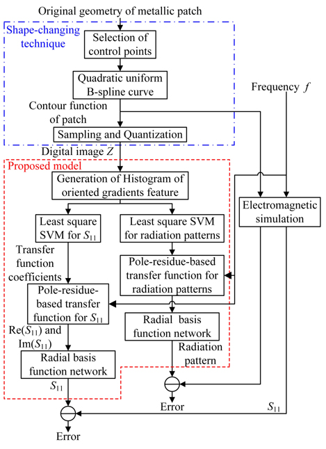
Figure 1: Structure of the proposed model and the shape-changing technique.
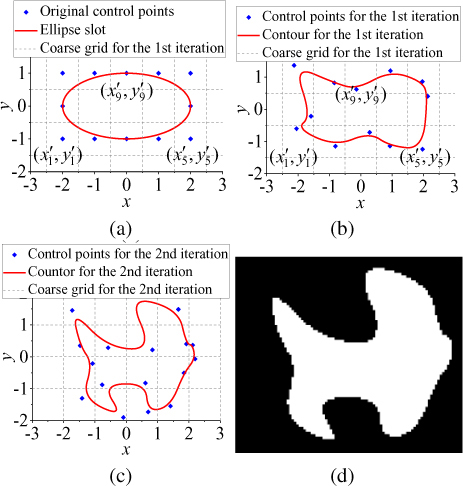
Figure 2: Diagram of the shape-changing technique for an ellipse slot: (a) Ellipse slot and the original control points, (b) control points and corresponding contour for the first iteration, (c) control points and corresponding contour for the second iteration, and (d) binary image Z.
For the ellipse slot, the corresponding curve for the circular control points is also shown in Fig. 2 (b).
In the next iteration, the coarse grid is shifted in both x- and y-directions by d/2. The control points are selected and shifted in a similar way again. In Fig. 2 (c), the positions of the grid lines are x = id and y = id, and a new contour is generated by (1) with square control points. The iteration process ends after the maximum number of iterations.
In sampling and quantization [10], the coordinate values are digitized to determine the pixel positions, and each material is denoted by specified numbers. In other words, the slot domain is discretized with a fine square gird, i.e., pixel, with the side length of d. The value of the pixels whose center lies inside the slot is 0, and the value of the others is 1.
B. Histogram of oriented gradients feature
Because the local object appearance and shape can be characterized well by the distribution of local intensity gradients or edge position, the histogram of oriented gradients feature is often used for human detection. In our model, the feature is used as the input of SVM to simply the relationship learned by the neural network.
The feature of the example is visualized over the slot image in Fig. 3. The extraction of the feature can be implemented by the MATLAB function extractHOGFeatures.
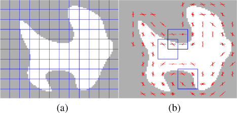
Figure 3: Extraction of histogram of oriented gradients features: (a) Binary image Z with cells, (b) visualization of the histogram of oriented gradients feature and blocks.
First, the gradient of each pixel is calculated. Second, the image is divided into small connected regions, i.e., cells, as shown in Fig. 3 (a). The size of cell is also defined based on the complexity of the slot contour and the training time. Then a local one-dimensional histogram of gradient directions over the pixels of the cell is accumulated for each cell. Nine bins are evenly spaced over the range of 0-180. To reduce aliasing, votes are interpolated bilinearly between the neighboring bin centers in both orientation and position. The vote of each pixel is the gradient magnitude. Fourth, the local histogram is contrast-normalized by a measure of the intensity across several cells, called a block, as shown in Fig. 3 (b). The number of overlapping cells between horizontally or vertically adjacent blocks is h v or h v, i.e., the block stride for the horizontal direction is h cells, and the one for the vertical direction is v cells. The block normalization scheme is Lowe-style clipped L2 norm. Then the histogram of oriented gradients feature vector is gotten. For an image with the pixel size of h v, the length N of the histogram of oriented gradients feature vector is
| (2) |
where the cell contains h v pixels and the block contains h v cells.
C. Multi-output least square SVM
To improve the reliability and accuracy of the whole model, the multi-output least square SVM [11] learns the mapping relation from the histogram of oriented gradients feature h to the transfer function coefficients c for electromagnetic responses (S or radiation patterns). The objective function of SVM and corresponding constrains are
| (3) |
where a radial basis function is used as the kernel function, i.e., (h)(h) = exp(-p||h- h||), p is a positive kernel scale parameter, weight matrix W = [w+ v, w+ v, …, ] (the smaller the w is, the more similar the transfer function coefficients are to each other), b is the bias vector, is the slack variable, and are the positive real regularized parameters, and m represents the number of training samples. Compared with CNN, there are much fewer hyper-parameters for the multi-output least square SVM, i.e., p, , and .
D. Pole-residue-based transfer function
The transfer function is employed to extract the feature of electromagnetic responses [5, 6]. The pole-residue-based transfer function coefficients have low sensitivities with respect to geometrical parameters, and they are a reasonable representation of electromagnetic responses. Thus, the neural network model based on the transfer function is accurate with high dimension of geometrical parameter space and large geometrical variations. The transfer function coefficients can be obtained with vector fitting [12]. The pole-residue-based transfer function is presented as
| (4) |
where p and r represent the pole and residue coefficients of transfer function, respectively, s is the frequency in Laplace domain, Q represents the order of transfer function, and the superscript * represents complex conjugate. The transfer function coefficient c is a vector of the real and imaginary part of p and r.
E. Radial basis function network
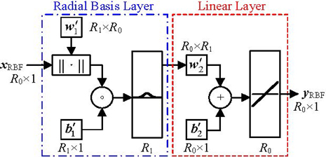
Figure 4: Structure of the radial basis function network.
The radial basis function network is used for error correction. It learns the relationship between the electromagnetic response (Sor radiation patterns) obtained from the transfer function and the simulated one. As shown in Fig. 4, there are two layers in the radial basis function network, i.e., a hidden radial basis layer with R neurons and an output linear layer with R neurons. The mathematical form is
| (5) |
where y is a vector of real and imaginary parts of electromagnetic responses, x is a vector of real and imaginary parts of H(s), denotes the Hadamard product, and are the weight vectors of the two layers, and and are the bias vectors of the two layers. This can be implemented by the MATLAB function newrb. The function newrb iteratively creates one more neuron for the radial basis function network. Neurons are added to the network until the mean squared error falls beneath a preset error goal or a maximum number of neurons is reached.
F. Training and optimization
In the training process, if the accuracy of the model is not acceptable, the hyper-parameters are adjusted or more training samples are added to retrain the model. The mean absolute percentage errors of the frequencies at |S| = -10 dB and the radiation pattern are adopted to measure calculation precision.
Once the model is trained, it can substitute the full-wave simulation and speed up the process of optimization. It is difficult to directly optimize the contour of slot in the image domain. The optimized variable is a vector of shifting distance in x- and y-directions for the control points.
III. APPLICATION EXAMPLE
A tri-passband microstrip-fed slot antenna [13] (see Fig. 5) is employed as an example to evaluate the proposed model. The original geometric parameters are as follows: W = 31 mm, L = 41 mm, W = 3.14 mm, L = 13.5 mm, l = 6.7 mm, l = 2.6 mm, t = 0.5 mm, s = 0.3 mm, D = 18 mm, D = 20 mm, d = 2.3 mm, d = 3.5 mm, w = 1.7 mm, and w = 4.1 mm. The metallic strips are printed on a substrate with a thickness of 1.59 mm and a relative permittivity of 4.4.
The slot shown in Fig. 5 (a) is considered for modeling, i.e., the first two resonant frequencies are modeled. The slot keeps mirror symmetry in both horizontal and vertical directions. Therefore, one-eighth of the slot is presented by a binary image, which contains 168 144 square pixels, i.e., h v = 168 144, with d = 0.05 mm. The metal and the substrate are denoted by 0 and 1, respectively. For the histogram of oriented gradients feature, h = 8, v = 8, h = 2, v = 2, h = 1, and v = 1. The length of the histogram of oriented gradients feature vector is 12,240.
HFSS 17.0 performs the full-wave simulation and generates training and testing samples; 400 training samples and 100 testing samples are defined randomly in Table 1. The control points are shifted in the blue polygon in Fig. 5 (c), and the geometric parameters of the blue polygon are l = 0.7 mm, l = 2 mm, l = 0.95 mm, l = 0.84 mm, l = 7.96 mm, and = 35.16. In the shape-changing process, the maximum iteration is 4 and the side length d of the coarse square gird for the samples is 0.8 mm.
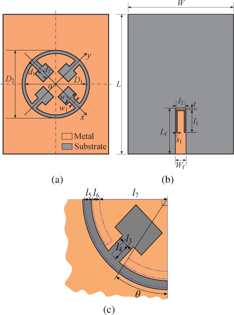
Figure 5: Geometry of the tri-passband microstrip-fed slot antenna: (a) Top view, (b) back view, (c) quarter slot.
Table 1: Definition of training and testing samples
| Training Data(400 Samples) | Testing Data(100 Samples) | |||||
| Min. | Max. | Step | Min. | Max. | Step | |
| x(mm) | -0.35 | 0.35 | 0.1 | -0.3 | 0.4 | 0.1 |
| y(mm) | -0.35 | 0.35 | 0.1 | -0.3 | 0.4 | 0.1 |
Table 2: Hyper-parameters of the trained SVM
| |S| | Patterns at the First Resonant Frequency | |||
|---|---|---|---|---|
| E Plane ( = [0, 180]) | E Plane ( = [180, 360]) | H Plane | ||
| p | 6.1710 | 5.9010 | 1.6210 | 8.8410 |
| 1.9110 | 2.4210 | 1.1710 | 1.0510 | |
| 8.9310 | 1.6210 | 1.9810 | 8.0510 | |
The hyper-parameters of the trained least square SVM are listed in Table 2, where the hyper-parameters are obtained with Bayesian optimization [14]. The training and testing errors for the frequencies at |S| = -10 dB and the radiation pattern (taking the pattern at the first resonant frequency for example) are given in Table 3. For comparison, a CNN model is also trained for the tri-passband antenna. The training and testing errors of the CNN model are at the same level as the proposed model. The training costs 1.1 mins for SVM, and 56.6 mins for CNN. Much less time is spent to train the proposed model, and fewer hyper-parameters need to be determined. For this paper, the calculations are performed on an Intel i5-1135G7 (2.4 GHz) machine with 16 GB RAM.
Table 3: Training and testing errors for the frequencies at |S| = -10 dB and the radiation patterns at the first resonant frequency
| Frequencies at |S| = -10 dB | Patterns at the First Resonant Frequency | |||
|---|---|---|---|---|
| Proposed Model | CNN Model | Proposed Model | CNN Model | |
| Training error | 0.13% | 0.48% | 0.96% | 0.85% |
| Testing error | 0.57% | 0.62% | 1.18% | 0.89% |
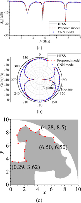
Figure 6: Comparison of the first testing sample: (a) |S|, (b) radiation patterns at the first resonant frequency, (c) image of a quarter of slot.
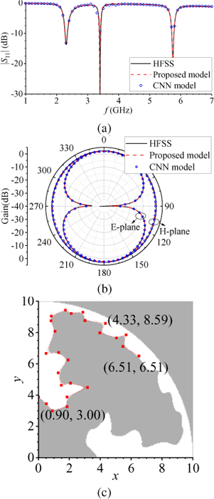
Figure 7: Comparison of the second testing sample: (a) |S|, (b) radiation patterns at the first resonant frequency, (c) image of a quarter of slot.
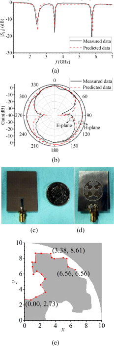
Figure 8: Optimization results for the example and photograph of the fabricated antenna: (a) |S|, (b) radiation patterns at the first resonant frequency, (c) top view, (d) back view, (e) image of a quarter of slot.
Two examples out of the training range are chosen to test the model, as shown in Figs. 6 and 7. The predicted electromagnetic responses of the proposed model and CNN model both agree well with the full-wave simulated ones from HFSS. The corresponding control points for the sample are shown in Figs. 6 (c) and 7 (c).
Once the model is trained, it can be applied to the optimization design as a substitute for the full-wave simulation. Then a tri-passband antenna is optimized with the genetic algorithm [15] to reach the design specification of |S| -10 dB (2.4-2.48 GHz, 3.49-3.54 GHz, and 5.72-5.79 GHz). From Fig. 8, the curves of predicted S-parameter and radiation pattern for the first resonant frequency agree well with the measured ones.
IV. CONCLUSION
In this paper, a new least square SVM model for shape modeling of slot antennas is proposed. In the modified shape-changing technique, the B-spline interpolation curve is used to describe the slot shape, and the corresponding slot image is used as the model input. The model consists of histogram of oriented gradients feature, transfer function, and the radial basis function network. The histogram of oriented gradients feature is extracted to obtain the distribution of local intensity gradients or edge position from the slot images. Then, the least square SVM maps the histogram of oriented gradients features into transfer function coefficients, and there are only three hyper-parameters that need to be determined in the training of SVM. The transfer function provides a preliminary prediction about electromagnetic response. In the end, the radial basis function network is applied to the error correction. A tri-passband microstrip-fed slot antenna is employed as an example to confirm the effectiveness of the proposed model. The proposed model gets the same precision as the CNN model while it costs much less trainingtime.
ACKNOWLEDGMENT
This work was supported by the National Natural Science Foundation of China under Grant 62171093 and by the Sichuan Science and Technology Programs under Grants 2022NSFSC0547 and 2022ZYD0109.
REFERENCES
[1] H. M. E. Misilmani, T. Naous, and S. K. A. Khatib, “A review on the design and optimization of antennas using machine learning algorithms and techniques,” Int. J. RF Microw. Comput.-Aided Eng., vol. 30, no. 10, p. e22356, Oct. 2020.
[2] L.-Y. Xiao, W. Shao, F.-L. Jin, and B.-Z. Wang, “Multiparameter modeling with ANN for antenna design,” IEEE Trans. Antennas Propag., vol. 66, no. 7, pp. 3718-3723, July 2018.
[3] T. Khan and C. Roy, “Prediction of slot-position and slot-size of a microstrip antenna using support vector regression,” Int. J. RF Microw. Comput.-Aided Eng., vol. 29, no. 3, p. e21623, Mar. 2019.
[4] Y. Kim, S. Keely, J. Ghosh, and H. Ling, “Application of artificial neural networks to broadband antenna design based on a parametric frequency model,” IEEE Trans. Antennas Propag., vol. 55, no. 3, pp. 669-674, Mar. 2007.
[5] F. Feng, C. Zhang, J. Ma, and Q.-J. Zhang, “Parametric modeling of EM behavior of microwave components using combined neural networks and pole-residue-based transfer functions,” IEEE Trans. Microw. Theory Techn., vol. 64, no. 1, pp. 60-77, Jan. 2016.
[6] F. Feng, V.-M.-R. Gongal-Reddy, C. Zhang, J. Ma, and Q.-J. Zhang, “Parametric modeling of microwave components using adjoint neural networks and pole-residue transfer functions with EM sensitivity analysis,” IEEE Trans. Microw. Theory Techn., vol. 65, no. 6, pp. 1955-1975, June 2017.
[7] J. P. Jacobs, “Accurate modeling by convolutional neural-network regression of resonant frequencies of dual-band pixelated microstrip antenna,” IEEE Antennas Wireless Propag. Lett., vol. 20, no. 12, pp. 2417-2421, Dec. 2021.
[8] H.-Y. Luo, W. Shao, X. Ding, B.-Z. Wang, and X. Cheng, “Shape modeling of microstrip filters based on convolutional neural network,” IEEE Microw. Wireless Compon. Lett., vol. 32, no. 9, pp. 1019-1022, Sep. 2022.
[9] N. Dalal and B. Triggs, “Histograms of oriented gradients for human detection,” IEEE Comput. Soc. Conf. Comput. Vis. Pattern Recognit., San Diego, CA, USA, vol. 1, pp. 886-893, 2005.
[10] R. C. Gonzalez and R. E. Woods, Digital Image Processing, USA: Prentice Hall, Upper Saddle River, NJ, 2002.
[11] S. Xu, X. An, X. Qiao, L. Zhu, and L. Li, “Multi-output least-squares support vector regression machines,” Pattern Recognit. Lett., vol. 34, no. 9, pp. 1078-1084, July 2013.
[12] B. Gustavsen and A. Semlyen, “Rational approximation of frequency domain responses by vector fitting,” IEEE Trans. Power Del., vol. 14, no. 3, pp. 1052-1061, July 1999.
[13] K. D. Xu, Y. H. Zhang, R. J. Spiegel, Y. Fan, W. T. Joines, and Q. H. Liu, “Design of a stub-loaded ring-resonator slot for antenna applications,” IEEE Trans. Antennas Propag., vol. 63, no. 2, pp. 517-524, Feb. 2015.
[14] J. Snoek, H. Larochelle, and R. P. Adams, “Practical Bayesian optimization of machine learning algorithms” in Adv. in Neural Inf. Process. Syst. 25, USA: Curran Associates Inc., Red Hook, NY, pp. 2951-2959, 2012.
[15] R. L. Haupt and D. H. Werner, Genetic Algorithms in Electromagnetics, USA: Wiley, Hoboken, NJ, 2007.
BIOGRAPHIES

Hai-Ying Luo received the B.S. degree from the University of Electronic Science and Technology of China (UESTC), Chengdu, China, in 2017, where he is currently pursuing the Ph.D. degree in radio physics.
His current research interest is computational electromagnetics.

Wen-Hao Su received the B.S. degree from UESTC, Chengdu, China, in 2021, where he is currently pursuing the master’s degree in radio physics.
His current research interests include antenna design and computational electromagnetics.

Haiyan Ou received the B.E. degree in electrical engineering from UESTC in 2000, and received Ph.D. degrees in optical engineering from Zhejiang University in 2009.
She joined UESTC in 2009 and is now an associate professor there. From 2010 to 2011, she was a visiting scholar in the department of Engineering, Cambridge University, UK. From 2012 to 2013, she was a post-doc in the Department of Electrical and Electronic Engineering, the University of Hong Kong. Her research interests include computational electromagnetics, microwave photonics, and digital holography.

Sheng-Jun Zhang received Ph.D. in science from Beijing University of Technology in 2001. From then on he joined the team in National Key Laboratory of Science & Technology on Test Physics and Numerical Mathematics. He is now professor of the laboratory and his research interests include scattering of EM waves, EM effects of periodic structures such as FSS, PC and gratings, as well as modulation of scattering of materials and interaction of EM waves with plasmas, IR radiation management.
He has published some papers in journals and conferences, in addition to patents and two books.

Wei Shao received the B.E. degree in electrical engineering from UESTC in 1998, and received M.Sc. and Ph.D. degrees in radio physics from UESTC in 2004 and 2006, respectively.
He joined UESTC in 2007 and is now a professor there. From 2010 to 2011, he was a visiting scholar in the Electromagnetic Communication Laboratory, Pennsylvania State University, State College, PA. From 2012 to 2013, he was a visiting scholar in the Department of Electrical and Electronic Engineering, the University of Hong Kong. His research interests include computational electromagnetics and antenna design.
ACES JOURNAL, Vol. 38, No. 9, 687–694
doi: 10.13052/2023.ACES.J.380908
© 2023 River Publishers