Outlier Detection-aided Supervised Learning for Modeling of Thinned Cylindrical Conformal Array

Yang Hong${}^{\mathbf{\text{1}}}$, Wei Shao${}^{\mathbf{\text{1}}}$, Yan He Lv${}^{\mathbf{\text{2}}}$, and Zhi Ning Chen${}^{\mathbf{\text{2}}}$

¹School of Physics
University of Electronic Science and Technology of China, Chengdu, 610054, China
yanghong@std.uestc.edu.cn, weishao@uestc.edu.cn
²Department of Electrical and Computer Engineering
National University of Singapore, Singapore, 117583, Singapore
aplyh@nus.edu.sg, eleczn@nus.edu.sg

Submitted On: February 27, 2023; Accepted On: June 13, 2023

ABSTRACT

In this paper, a scheme of outlier detection-aided supervised learning (ODASL) is proposed for analyzing the radiation pattern of a thinned cylindrical conformal array (TCCA), considering the impact of mutual coupling. The ODASL model has the advantage in speed improvement and memory consumption reduction, which enables a quick generation of the synthesis results with good generalization. The utilization of the active element pattern (AEP) technique in the model also contributes to the prediction of the array performance involving mutual coupling. The effectiveness of the ODASL model is demonstrated through a numerical example of the 12-element TCCA.

Index Terms: Active element pattern (AEP), conformal array, outlier detection-aided supervised learning (ODASL), thinned array.

I. INTRODUCTION

Recently, conformal arrays have gained popularity in airborne and satellite applications for the sake of their adaptability and aerodynamic performance. However, their analysis and synthesis are particularly complicated due to the varying positions and axial directions of the elements [1]. In addition, the impact of mutual coupling between elements makes it difficult to analyze the far field of conformal arrays, using the directional product theorem applied to planar arrays [2].

The supervised learning method has been extensively recognized as a prediction tool with significant improvement and contribution to electromagnetic (EM) modeling [3–5]. It provides a fast synthesis process for array behaviors while maintaining high-level accuracy with a reduced number of full-wave simulations. However, a multitude of inner parameters of a supervised learning method needs to be determined for large-space and high dimensional problems [6, 7], which easily makes learning progress tardy. In addition, the dependence on sampling data may affect the credibility of the model, especially in the context of array modeling with a complex structure and EM environment. To solve this problem, outlier detection (OD) in data mining is explored as an effective decision-making tool [8]. The multivariate distance-based OD method is used to traverse the raw dataset and identify outlier objects, helping to construct the model effectively.

Considering the impact of mutual coupling and array environment on radiation patterns, a large-scale array can be transformed into the superposition of small sub-arrays by employing the active element pattern (AEP) technique [9]. The technique offers attractive benefits, including the avoidance of heavy calculation burden associated with the whole-array simulation.

To make better use of sampling data, this paper proposes an outlier detection-aided supervised learning (ODASL) model as an alternative to the costly measurement or full-wave simulation. Considering mutual coupling and EM environment, the AEP technique is employed to extract the patterns of sub-arrays, instead of the whole array. By filtering out the invalid sampling data, i.e., outlier data, the ODASL model can obtain satisfactory prediction results, with a strong generalization ability even for larger thinned cylindrical conformal array (TCCA) scales. A TCCA is taken as an example to demonstrate the effectiveness of the proposed model.

II. PROPOSED METHODOLOGY

A. Definition and realization of outlier identification

In the regression supervised learning method for EM modeling, the learning information is completely sourced from the sampling dataset. Hence, it is necessary to perform OD on the raw dataset for the analysis to accurately construct the ODASL framework. The training dataset $\mathit{T}$, defined as $\{{\mathit{S}}_1,{\mathit{S}}_2,\mathrm{\dots },{\mathit{S}}_D\}$, contains a total of $D$ labeled samples, and the EM response denoted as $\mathit{y}$ in each sample is obtained from full-wave simulations. Assuming that there are $M$ uncertain outlier samples in the raw training dataset, they can be recorded as $\mathit{O}=[{\mathit{O}}_1,{\mathit{O}}_2,\mathrm{\dots }{\mathit{O}}_{M-1},{\mathit{O}}_M]$. To measure the similarity in distance between a pair of data objects ${\mathit{S}}_j$ and ${\mathit{S}}_k$, a distance function is defined as $\mathit{\text{dis}}({\mathit{S}}_j,{\mathit{S}}_k)$, satisfying the positive definiteness: $\mathit{\text{dis}}({\mathit{S}}_j,{\mathit{S}}_k)⩾0$, shown as

$$\mathit{\text{dis}}({\mathit{S}}_j,{\mathit{S}}_k)=\sum _{1⩽t⩽L}{\left(\right|y_{{\mathit{S}}_j,t},y_{{\mathit{S}}_k,t}{|}^q)}^{1/q},q⩾1$$

(1)

where $L$ represents the number of sampling points in $\mathit{y}$ for each sample, $y_{S_{j,t}}$ and $y_{{\mathit{S}}_k,t}$ are the the sampling point values for samples ${\mathit{S}}_j$ and ${\mathit{S}}_k$, respectively. Generally, the Euclidean distance, which is the second-order Minkowski distance with $q=2$ in formula (1), is adopted as the calculation method to ensure the stability of results regardless of the variation of the dataset space.

With the aid of the transfer function (TF) [10], poles $\mathit{p}$ and residues $\mathit{r}$, which are TF coefficients to describe behaviors of samples, are extracted as the corresponding measurement values and used to identify outliers. The implementation of the specific steps in the OD stage shown in Fig. 1, is described as follows:

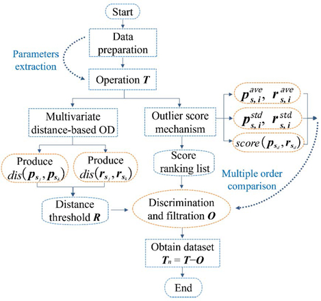
Figure 1: Flow diagram of outlier identification mechanism.

1. Step 1: For each sample in $\mathit{T}$, the full-wave simulation of the EM response target $\mathit{y}$, representing the results obtained with AEP, is completed in the range of the specified geometric parameters. The results obtained from the frequency-domain analysis are then fitted to poles/residues-based transfer functions utilizing the vector fitting (VF)technique [11].

2. Step 2: The TF coefficients extracted from all samples have the same order $N$, and the poles of a sample ${\mathit{S}}_d$ are set as ${\mathit{p}}_{{\mathit{S}}_d}=(p_{{\mathit{S}}_d,1},p_{{\mathit{S}}_d,2},\mathrm{\dots },p_{{\mathit{S}}_d,i},\mathrm{\dots },p_{{\mathit{S}}_d,N})$. Similarly, the residues of ${\mathit{S}}_d$ are represented by ${\mathit{r}}_{{\mathit{S}}_d}=(r_{{\mathit{S}}_d,1},r_{{\mathit{S}}_d,2},\mathrm{\dots },r_{{\mathit{S}}_d,i},\mathrm{\dots },r_{{\mathit{S}}_d,N})$, where $d=1,2,\mathrm{\dots },D,i=1,2,\mathrm{\dots },N,p_{{\mathit{S}}_d,i}$ and $r_{{\mathit{S}}_d,i}$ are the pole and residue values of the ith order of ${\mathit{S}}_d$, respectively. $p_{{\mathit{S}}_{d,i}}$ and $r_{{\mathit{S}}_d,i}$ in the dataset are clustered according to their corresponding order. For the calculation of $\mathit{\text{dis}}({\mathit{S}}_j,{\mathit{S}}_k)$, it is converted to the calculation of the accumulation of two-part distances: one is related to $\mathit{p}$ expressed as $\mathit{\text{dis}}({\mathit{p}}_{{\mathit{S}}_j},{\mathit{p}}_{{\mathit{S}}_k})={\sum }_{1⩽i⩽N}\mathit{\text{dis}}(p_{{\mathit{S}}_{j,}i},p_{{\mathit{S}}_k,i})$, and another is $\mathit{\text{dis}}({\mathit{r}}_{S_j},{\mathit{r}}_{S_k})={\sum }_{1⩽i⩽N}\mathit{\text{dis}}(r_{S_i,i},r_{S_k,i})$ for $\mathit{r}$.

3. Step 3: The given dataset $\mathit{T}$ is evaluated by $a$) To distinguish obvious outliers unequivocally, the distances of $\mathit{\text{dis}}({\mathit{p}}_{S_j},{\mathit{p}}_{S_k})$ and $\mathit{\text{dis}}({\mathit{r}}_{S_j},{\mathit{r}}_{S_k})$ with the same order are subject to a restrictive distance threshold $\mathit{R}=[{\mathit{R}}_{{\mathit{p}}_{\mathrm{dis}}},{\mathit{R}}_{{\mathit{r}}_{\mathrm{dis}}}]$, with a dimension of $2N\times 1$. The threshold varies with different sampling datasets. $b$) Intrinsically, due to the interdependence among the data points, detecting micro-clusters becomes more complex as these outliers may be neglected as data points from the dense regions of data distribution. Therefore, the outlier score mechanism (OSM) is adopted,denoted as

$$\mathit{\text{score}}({\mathit{p}}_{{\mathit{S}}_d},{\mathit{r}}_{{\mathit{S}}_d})=\sum _i^N\mathit{\text{score}}(p_{{\mathit{S}}_d,i},r_{{\mathit{S}}_d,i}),$$

(2)

where

$$\mathit{\text{score}}(p_{{\mathit{S}}_d,i},r_{{\mathit{S}}_d,i})=\parallel \frac{p_{{\mathit{S}}_d,i}-p_{\mathit{S},i}^{\mathit{\text{ave}}}}{p_{\mathit{S},i}^{\mathit{\text{std}}}},\frac{r_{{\mathit{S}}_d,i}-r_{\mathit{S},i}^{\mathit{\text{ave}}}}{r_{\mathit{S},i}^{\mathit{\text{std}}}}\parallel ,$$

(3)

where $p_{s,i}^{ave}$ and $r_{s,i}^{ave}$ are the average values of the ith order pole and residue, respectively, $p_{s,i}^{std}$ and $r_{s,i}^{std}$ represent the standard deviation. The absolute value of the score indicates the distance between the data points and the population averages, within the scope of the standard deviation. By filtering out samples with outlier points, a collection of outlier samples $\mathit{O}$ is obtained, and the remained dataset is ${\mathit{T}}_n=\mathit{T}-\mathit{O}$.

To sum up, the approach for analyzing and identifying outliers can be accomplished by choosing the top $M$ outliers with the largest outlier scores from the score ranking list and by selecting outliers from a cut-off threshold, depending on the distribution ofoutliers.

B. Proposed ODASL for array modeling

Taking the parametric modeling of arrays for example, the specific procedure with various stages of the ODASL model is presented in Fig. 2. The overall input $\mathit{x}$ consists of geometric parameters of the element and element spacing. In practice, we want to obtain the relationship between variables in $\mathit{x}$ and EM response $\mathit{y}$ that is affected by mutual coupling and array environment. For exploring the relationship of labeled data pairs of $(\mathit{x},\mathit{y})$, we have

$$f:V_{\mathit{x}}\to V_{\mathit{y}},$$

(4)

where $f$ is the nonlinear function for the mapping of input space $V_{\mathit{x}}$ to output space $V_{\mathit{y}}$. In the whole set, $V_{\mathit{x}}$ and $V_{\mathit{y}}$ cannot be traversed completely because of the limitation of the sampling requirement, expressed by

$$f\left(V_{\mathit{x}}\right)=\{f(\mathit{x}):\mathit{x}\in V_{\mathit{x}}\}\subseteq V_{\mathit{y}}.$$

(5)

In Phase I of the ODASL architecture, dataset generation is the first step to provide the samples for modeling. According to the modeling requirement, the EM response is set as the target, such as $S_{11}$ or pattern information. Then the next step is to obtain the samples with the variable geometric structure and element spacings from the full-wave simulation, and to extract the relevant TF coefficients from EM response.

In Phase II, the potential outliers in $\mathit{T}$ are filtered out using the previous process, and then the input samples of ${\mathit{T}}_n$ are obtained. For the output, the sub-array patterns based on TF coefficients are accurately captured by the AEP technique. According to the positions of elements, they are categorized into edge element, adjacent-edge element, and interior element, and their AEPs are extracted separately [12, 13].

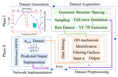
Figure 2: Overall architecture of the ODASL model.

Subsequently, in the training process of the multi-branch radial basis function neural network (RBFNN) [14], by adjusting the network parameters of multi-branch RBFNN, including the weights of hidden/output layer and center/width of basis function, the relationships between the input and the output in three branches are established. The main purpose of training is to minimize the disparity between $\mathit{y}$ and the predicted $\overline{\mathit{y}}$ from the superposition of all branch results.

To test the model, its generalization ability is crucial to the stable prediction, especially for input $\mathit{x}$ beyond the range of the training dataset [15]. Combined with AEP, a high-degree freedom of array design is guaranteed, and the time-consuming full-wave simulation for the whole array is substituted by the superposition of the predictions from multi-branch networks for sub-arrays. Once the proposed model is well-trained, it immediately provides an accurate response for a given input.

III. NUMERICAL RESULT

A 12-element TCCA in Fig. 3 is taken as the example to evaluate the ODASL model, where it works at $3.5\mathrm{GHz}$ [16]. The elements are placed on a cylindrical substrate with a radius $r_{\mathrm{a}}=800\mathrm{mm}$ and a relative dielectric constant of ${\epsilon }_{\mathrm{r}}=2.65$. To obtain a high degree of freedom, the input is denoted as $\mathit{x}={[L_{\mathrm{x}},W_{\mathrm{y}},W_{\mathrm{l}},L_{\mathrm{a}},W_{\mathrm{b}},f_{\mathrm{x}},\mathit{d}]}^{\mathrm{T}}$, extracted with the design of the experiment method for sampling [17]. The circumferential distance in $\mathit{d}={[d_1,d_2,\mathrm{\dots },d_e]}^{\mathrm{T}}$ is approximately from $0.43\lambda$ to $0.54\lambda$ during the data collection, where $e$ is equal to 2, 3, or 4 for AEP extraction, depending on the sub-array scale. Table 1 shows the sampling data for the branch of the adjacent-edge element. Data values are standardized before they are used in the network. Similarly, 81 training samples and 36 testing samples are collected for edge elements, and 100 training samples and 64 testing samples are collected for interior elements.

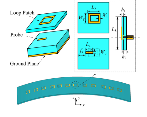
Figure 3: Structure of the 12-element TCCA, with top, back, and cross-sectional views of the planar surface.

Table 1: Definition of training and testing data for adjacent-edge elements (unit: $\mathrm{mm}$)

Structure Parameter	Training Dataset (100 Samples)			Testing Dataset (49 Samples)
	Min	Max	Step	Min	Max	Step
$L_{\mathrm{x}}$	18	22.5	0.5	18.6	21.6	0.5
$W_{\mathrm{y}}$	13	17.5	0.5	13.8	16.8	0.5
$W_1$	1.75	2.2	0.05	1.82	2.12	0.05
$L_{\mathrm{a}}$	5.6	6.5	0.1	5.75	6.35	0.1
$W_{\mathrm{b}}$	1.5	2.4	0.1	1.65	2.25	0.1
$f_{\mathrm{x}}$	-8.5	-7.4	0.1	-8.75	-7.35	0.1
$d_i$	37	46	1	38.5	44.5	1

To predict the array pattern considering mutual coupling, firstly, the AEPs of all elements are extracted from the raw data, and the corresponding ${\mathit{p}}_{{\mathit{S}}_d}$ and ${\mathit{r}}_{{\mathit{S}}_d}$ are obtained. All collected raw datasets are operated in OD processing, and the distances of $\mathit{p}$ and $\mathit{r}$ for each order are acquired, with the maximum order $N=12$. Secondly, the correlated values of the OSM in formula (3) are calculated, and the scores of each sample are ranked in terms of their degree of deviation. For outlier samples, the distance exceeds the threshold, and meanwhile, the level of outliers is relatively obvious. An example of OD processing for edge elements in the training process is displayed in Table 2, where the values of $\mathit{R}$ and score ranking for each order are exhibited.

Further, Table 3 embodies the situations of $M=13$ outlier samples, with a certain order of $\mathit{p}$ or $\mathit{r}$ in ${\mathit{S}}_{\mathit{\text{dis,i}}}$ over $\mathit{R}$ and a high degree of dispersion score, where ${\mathit{S}}_{\mathit{\text{dis, i}}}$ is the $i$th distance between $\mathit{\text{dis}}(p_{{\mathit{S}}_{s,i}},p_{{\mathit{S}}_k,i})$ and $\mathit{\text{dis}}(r_{{\mathit{S}}_{s,i}},r_{{\mathit{S}}_k,i})$ for the outliers. Similarly, performing the same operations on all element categories, the resulting filtered sets are used as the branch target outputs.

Table 2: Definition of the parameters of OD processing of the training data for edge elements

Order	1	2	3	4	5	6
$R_{{\mathit{p}}_{\mathrm{dis}},i}$	0.71	0.87	0.55	0.68	0.89	2.87
$R_{{\mathit{r}}_{\mathrm{dis}},i}$	2.18	2.91	3.62	2.13	6.57	2.29
$p_{\mathit{S},i}^{ave}$	0.35	0.46	0.69	1.61	2.42	3.54
$r_{\mathit{S},i}^{ave}$	0.37	0.49	1.41	-0.98	3.77	0.21
$p_{\mathit{S},i}^{std}$	0.25	0.35	0.82	0.17	0.14	0.09
$r_{{\mathit{S}}_i}^{std}$	1.31	1.15	1.52	0.81	2.20	0.83
Order	7	8	9	10	11	12
$R_{{\mathit{p}}_{\mathrm{dis}},i}$	0.29	0.55	0.48	1.76	0.87	0.45
$R_{{\mathit{r}}_{\mathrm{dis}},i}$	1.87	1.48	2.12	4.61	1.12	1.83
$p_{\mathit{S},i}^{ave}$	-0.31	-0.42	0.45	2.23	1.08	0.74
$r_{\mathit{S},i}^{ave}$	-0.11	-0.85	1.44	1.25	0.82	0.55
$p_{\mathit{S},i}^{std}$	0.13	0.06	0.05	0.08	0.14	0.06
$r_{\mathit{S}i}^{std}$	1.10	0.84	0.53	2.19	0.25	0.37

Table 3: Outlier samples identified of the training dataset for edge elements

No. of Outlier	Outlier Order		${\mathit{S}}_{\mathit{d}\mathit{i}\mathit{s}\mathbf{,}\mathit{i}}$	$\mathit{S}\mathit{c}\mathit{o}\mathit{r}\mathit{e}$
	Index	$\mathbf{p}/\mathbf{r}$
1	4	$r$	3.52	3.38
2	7	$r$	2.91	1.41
3	4	$r$	3.26	3.32
4	6	$p$	3.72	2.30
5	11	$r$	1.10	2.78
6	10	$p$	2.49	2.80
7	4	$r$	1.25	3.09
8	7	$r$	2.63	1.26
9	1	$p$	1.18	5.29
10	10	$p$	2.27	2.72
11	11	$r$	1.06	2.71
12	7	$r$	2.42	1.15
13	5	$p$	1.21	2.21

Assisted by the characteristics of RBFNN, fast learning speed and high accuracy, the ODASL model predicts the pattern promptly from the three branches, avoiding full-wave EM simulations of the whole array. Furthermore, the predicted results can be written as

$${\mathit{E}}_{\text{total}}={\mathit{E}}_{\mathrm{e}}(\theta ,\phi )+{\mathit{E}}_{\mathrm{a}}(\theta ,\phi )+{\mathit{E}}_{\mathrm{i}}(\theta ,\phi )$$

(6)

where ${\mathit{E}}_{\mathrm{e}}(\theta ,\phi ),{\mathit{E}}_{\mathrm{a}}(\theta ,\phi )$, and ${\mathit{E}}_{\mathrm{e}}(\theta ,\phi )$ represent the fields acquired from the proposed ODASL model of all the edge elements, adjacent-edge elements, and interior elements, respectively.

To describe the above formula, ${\mathit{E}}_{\mathrm{e}}(\theta ,\phi )$ is shown as an example:

$${\mathit{E}}_{\mathrm{e}}(\theta ,\phi )=\sum _{1⩽s⩽N_{\mathrm{e}}}{I}_s{\mathit{F}}_s^{\mathrm{e}}(\theta ,\phi ){\mathrm{e}}^{jk\widehat{\mathit{r}}\cdot \mathit{r}s}$$

(7)

where $I_{\mathrm{s}}$ refers to the excitation amplitude of the sth edge element, $N_{\mathrm{e}}$ is the number of edge elements, ${\mathit{F}}_s^{\mathrm{e}}(\theta ,\phi )$ is the AEP result of the sth edge element, $k=2\pi /\lambda$ is the wavenumber in free space, where $\lambda$ is the wavelength, and ${\mathrm{e}}^{\mathrm{j}k\widehat{\mathit{r}}\cdot \mathit{r}s}$ is the spatial phase factor. Accordingly, the far-field pattern of the TCCA is obtained by superimposing the extracted results.

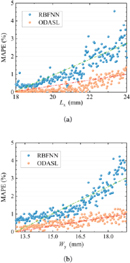
Figure 4: Pattern results of the proposed model and the full-wave simulation at 3.5 GHz: (a) Array 1 and (b) Array 2.

Accordingly, after the OD process filters out 13 training and 6 testing outlier samples for edge elements, 15 training and 7 testing samples for adjacent-edge elements, and 16 training and 10 testing samples for interior elements, the construction of the ODASL model for the 12-element TCCA costs approximately 13.92 hours, and the average mean absolute percent errors (MAPEs) of the training and testing processes for the whole proposed ODASL model are $3.576\%$ and 4.358%, respectively. All calculations are performed on an Intel i7-6700 3.40 GHz machine with 16 GB RAM.

As an example of TCCA modeling, the results of two separate arrays are shown in Fig. 4. For Array 1, the parameters of input ${\mathit{x}}_1$ are within the training dataset range, while those of input ${\mathit{x}}_2$ in Array 2 are outside the range: The parameters of ${\mathit{x}}_1=[19.2,17.7,1.84,6.32,2.03,-8.44,37.5,39.4,37.7,$ $40.1,38.6,44.2,38.5,37.2,38.3,40.7,39.8]{}^{\mathrm{T}}$, with a MAPE value 3.317%, and ${\mathit{x}}_2=[23.2,18.3,2.$ $57,7.1,2.26,-8.9,36.5,36.9,46.4,36.7,46.2,35.8,36.2$, 46.3, 36.8, 46.1, 36.6]${}^{\mathrm{T}}$, with a MAPE value 4.334%. From Fig. 4, the obtained agreement between the simulation and the ODASL model results proves the advantage of the proposed model in terms of accuracy for input parameters both within and outside the training dataset range.

To reflect the properties of the ODASL model with the TF coefficients as the outputs by extracting the AEPs from the sub-arrays, it is compared with the efficient extreme learning machine (ELM) [18, 19] and RBFNN, which directly output the whole array performance without involving the AEP technique. Table 4 indicates the network structure and computational accuracy of the three models. The error measurement standards include MAPE and root mean square error (RMSE), and the small MAPE and RMSE values of ODASL show its well-predicted performance in accuracy and stability. The ELM and RBFNN models collect 49 training samples and 25 testing samples within the parameter range in Table 1.

Table 4: Comparison of the three different models

	TF Order	No. of Hidden Neurons	MAPE	RMSE
RBFNN	17	23	$7.92\%$	0.0125
21	30	$6.69\%$	0.0093
ELM	17	10	$6.24\%$	0.0076
21	15	$5.71\%$	0.0052
ODASL	12	$7;7;8$	$3.58\%$	0.0029
14	$10;11;12$	$3.06\%$	0.0018

The ELM and RBFNN models use a single hidden layer, with 17 inputs, including the structure parameters and non-uniform element spacings. Here two cases of different TF orders are employed for TCCA modeling.

From Table 4, the proposed ODASL model shows lower errors than those of ELM and RBFNN for the two cases. In other words, more collected samples for the training of ELM and RBFNN are needed to get the same level of accuracy.

To examine the applicability of the OD process in the proposed model, Table 5 provides the error comparison for the multi-branch RBFNN model and the ODASL model, which are based on the same dataset obtained from the AEP technique. It is shown that even though the network structures for the two models are similar, the proposed model yields more accurate results.

Table 5: Comparison between the proposed ODASL model and the multi-branch RBFNN model

	Element	Category	ODASL Model	Multi-branch RBFNN Model
	Training Error	Testing Error	Training Error	Testing Error
Edge	$0.894\%$	$0.923\%$	$1.272\%$	$1.709\%$
Adjacent-edge	$0.952\%$	$1.106\%$	$1.744\%$	$2.235\%$
Interior	$1.137\%$	$1.194\%$	$2.405\%$	$2.928\%$

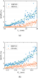
Figure 5: Comparison of MAPE results with varying parameters: (a) $L_{\mathrm{x}}$ and (b) $W_{\mathrm{y}}$.

In Fig. 5 (a), the predicted MAPEs of the multi-branch RBFNN and the proposed model are compared, where the parameter of $L_{\mathrm{x}}$ is considered as a single variable of the array. Figure 5 (b) provides the results of the parameter of $W_{\mathrm{y}}$. The results show that within the training dataset range, the proposed model gets satisfactory results. Even if the input parameter is out of the range of the training dataset, the proposed model can obtain much more accurate results than the multi-branch RBFNN model.

For further comparison, the proposed ODASL model, full-wave simulation, multi-branch RBFNN and ELM are employed to simulate a 22-element array, a 46-element array, and a 75-element array. The CPU time is listed in Table 6. Compared with the full-wave simulation, the ODASL model is constructed at a cost of 13.9 hours. For large scale arrays, however, the well-trained ODASL can be re-called to realize the fast simulation. Because ELM does not involve the AEP technique, three ELM models corresponding to the different array scales are constructed. Thus the whole modeling time with ELM is much more than that with ODASL. Compared with the multi-branch RBFNN combined with the AEP technique, the ODASL model filters out the invalid sampling data. Therefore, ODASL needs fewer training samples than the multi-branch RBFNN, and then it shows higher modeling efficiency.

Table 6: Comparison of CPU time for different arrays

Number of Elements	$\mathbf{22}$	$\mathbf{46}$	$\mathbf{75}$
Full-wave Simulation	$\mathrm{CT}$	–	–	–
	RT	$3.3\mathrm{h}$	$8.4\mathrm{h}$	$19.0\mathrm{h}$
	Total	$30.7\mathrm{h}$
ELM	$\mathrm{CT}$	$14.3\mathrm{h}$	$16.2\mathrm{h}$	$20.2\mathrm{h}$
	RT	$1.2\mathrm{m}$	$1.5\mathrm{m}$	$1.6\mathrm{m}$
	Total	$50.8\mathrm{h}$
Multi-branch RBFNN	$\mathrm{CT}$	$26.2\mathrm{h}$	–	–
	RT	$1.8\mathrm{m}$	$2.1\mathrm{m}$	$2.7\mathrm{m}$
	Total	$26.3\mathrm{h}$
ODASL	CT	$13.9\mathrm{h}$	–	–
	RT	$1.2\mathrm{m}$	$1.4\mathrm{m}$	$1.5\mathrm{m}$
	Total	$14.0\mathrm{h}$
CT/RT: Construction/Running time, h: hour, m: minute

IV. CONCLUSION

In this paper, a novel ODASL framework is proposed for efficient TCCA modeling, addressing the challenge posed by mutual coupling and data dependence, with the aim of meeting high-performance requirements for radiation pattern prediction. The proposed model provides a fast pattern realization process with an appreciable reduction of full-wave EM simulations. Combined with the AEP technique, the OD method employs multivariate distance-based clustering and OSM to enhance the discernment and quantification of outliers, constructing the operation for a highgeneralizable model. The valid samples are obtained by outlier elimination, and a numerical example demonstrates the effectiveness of the ODASL model. Additionally, the proposed model with the related data mining method can be further extended to other microwave applications.

ACKNOWLEDGMENT

This work was supported by the National Natural Science Foundation of China under Grant 62171093 and by the Sichuan Science and Technology Programs under Grants 2022NSFSC0547 and 2022ZYD0109.

REFERENCES

[1] J. Harris and H. Shanks, “A method for synthesis of optimum directional patterns from nonplanar apertures,” IRE Trans. Antennas Propag., vol. 10, no. 3, pp. 228-236, May 1962.

[2] L. I. Vaskelainen, “Constrained least-squares optimization in conformal array antenna synthesis,” IEEE Trans. Antennas Propag., vol. 55, no. 3, pp. 859-867, Mar. 2007.

[3] C. A. Oroza, Z. Zhang, T. Watteyne, and S. D. Glaser, “A machine-learning-based connectivity model for complex terrain large-scale low-power wireless deployments,” IEEE Trans. Cognit. Commun. Netw., vol. 3, no. 4, pp. 576-584, Dec. 2017.

[4] L.Y. Xiao, W. Shao, F. L. Jin, B. Z. Wang, and Q. H. Liu, “Inverse artificial neural network for multiobjective antenna design,” IEEE Trans. Antennas Propag., vol. 69, no. 10, pp. 6651-6659, Oct. 2021.

[5] P. Liu, L. Chen, and Z. N. Chen, “Prior-knowledge-guided deep-learning-enabled synthesis for broadband and large phase shift range metacells in metalens antenna,” IEEE Trans. Antennas Propag., vol. 70, no. 7, pp. 50245034, July 2022.

[6] A. Seretis and C. D. Sarris, “An overview of machine learning techniques for radiowave propagation modeling,” IEEE Trans. Antennas Propag., vol. 70, no. 6, pp. 3970-3985, June 2022.

[7] R. Caruana, N. Karampatziakis, and A. Yessenalina, “An empirical evaluation of supervised learning in high dimensions,” Proc. 25th Int. Conf. Mach. Learn., pp. 96-103, 2008.

[8] H. Wang, M. J. Bah, and M. Hammad, “Progress in outlier detection techniques: A survey,” IEEE Access, vol. 7, pp. 107964-108000, Aug. 2019.

[9] D. F. Kelley and W. L. Stutzman, “Array antenna pattern modeling methods that include mutual coupling effects,” IEEE Trans. Antennas Propag., vol. 41, no. 12, pp. 1625-1632, Dec. 1993.

[10] F. Feng, C. Zhang, J. Ma, and Q. J. Zhang, “Parametric modeling of EM behavior of microwave components using combined neural networks and pole-residue-based transfer functions,” IEEE Trans. Microw. Theory Techn., vol. 64, no. 1, pp. 60-77, Jan. 2016.

[11] B. Gustavsen and A. Semlyen, “Rational approximation of frequency domain responses by vector fitting,” IEEE Trans. Power Del., vol. 14, no. 3, pp. 1052-1061, July 1999.

[12] Q. Q. He and B.-Z. Wang, “Design of microstrip array antenna by using active element pattern technique combining with Taylor synthesis method,” Prog. Electromagn. Res., vol. 80, pp. 63-76,2008.

[13] Y. Hong, W. Shao, Y. H. Lv, B. Z. Wang, L. Peng, and B. Jiang, “Knowledge-based neural network for thinned array modeling with active element patterns,” IEEE Trans. Antennas Propag., vol. 70, no. 11, pp. 11229-11234, July 2022.

[14] F. Feng, W. Na, J. Jin, J. Zhang, W. Zhang, and Q. J. Zhang, “Artificial neural networks for microwave computeraided design: The state of the art,” IEEE Trans. Microw. Theory Techn., vol. 70, no. 11, pp. 4597-4619, Nov. 2022.

[15] H. Kabir, Y. Cao, and Q. J. Zhang, “Advances of neural network modeling methods for RF/ microwave applications,” Applied Computational Electromagnetics Society (ACES) Journal, vol. 25, no. 5, pp. 423-432, May 2010.

[16] Y. Kimura, S. Saito, Y. Kimura, and T. Fukunaga, “Design of wideband multi-ring microstrip antennas fed by an L-probe for single-band and dual-band operations,” Proc. 2020 IEEE AP-S. Int. Symp, pp. TU-A1.4A.8, July 2020.

[17] R. Schmidt and R. G. Launsby, “Understanding Industrial Designed Experiments,” Colorado Springs, CO, USA: Air Force Academy, 1992.

[18] L.Y. Xiao, W. Shao, S. B. Shi, and B. Z. Wang, “Extreme learning machine with a modified flower Pollination algorithm for filter design,” Applied Computational Electromagnetics Society (ACES) Journal, vol. 23, no. 3, pp. 279-284,2018.

[19] B. Deng, X. Zhang, W. Gong, and D. Shang, “An overview of extreme learning machine,” Proc. 4th Int. Conf. Control Robot. Cybern. (CRC), pp. 189-195, Sep. 2019.

BIOGRAPHIES

Yang Hong received the B.S. degree in electronic information science and technology from the University of Electronic Science and Technology of China (UESTC), Chengdu, China, in 2017. Currently, she is working toward the Ph.D. degree in physics at UESTC. In 2022, she joined the Department of Electrical and Computer Engineering, National University of Singapore, Singapore, as a visiting student.

Her research interest is neural network, antenna array, and computational electromagnetics.

Wei Shao received the B.E. degree in electrical engineering from UESTC in 1998, and received M.Sc. and Ph.D. degrees in radio physics from UESTC in 2004 and 2006, respectively.

He joined UESTC in 2007 and is now a professor there. From 2010 to 2011, he was a visiting scholar in the Electromagnetic Communication Laboratory, Pennsylvania State University, State College, PA. From 2012 to 2013, he was a visiting scholar in the Department of Electrical and Electronic Engineering, the University of Hong Kong. His research interests include computational electromagnetics and antenna design.

Yan-he Lv received the B.S. degree and Ph.D. degree in electronic information science and technology and radio physics from UESTC in 2017 and 2022, respectively.

He is currently a Research Fellow in the National University of Singapore, Singapore. His main research interests include metasurface, phased array, time-reversed electromagnetic, and computational electromagnetics.

Zhi Ning Chen received the B.Eng., M.Eng., and Ph.D. degrees in electrical engineering from the Institute of Communications Engineering (ICE), China, in 1985, 1998, and 1993, and a second Ph.D. degree from the University of Tsukuba, Tsukuba, Japan in 2003.

He joined the National University of Singapore in 2012 as a tenured full professor. From 1988 to 1995, He was a lecturer and later a professor with ICE and a post-doctoral fellow and later an associate professor with Southeast University, Nanjing, China. From 1995 to 1997, he was a research assistant and later a research fellow with the City University of Hong Kong, Hong Kong. In 2001 and 2004, he visited the University of Tsukuba twice under the JSPS Fellowship Program (senior fellow). In 2004, he joined the IBM Thomas J. Watson Research Center, Ossining, NY, USA, as an academic visitor. In 2013, he joined the “Laboratoire des SignauxetSystèmes,” UMR8506 CNRS-Supelec-University Paris Sud, Gif-sur-Yvette, France, as a senior DIGITEO guest scientist. In 2015, he joined the Center for Northeast Asian Studies, Tohoku University, Sendai, Japan, as a senior visiting professor.

He was elevated a Fellow of the IEEE for the contribution to small and broadband antennas for wireless applications in 2007 and a Fellow of the Academy of Engineering, Singapore, in 2019 for the contribution to research, development, and commercialization of wireless technology.

He is pioneering in developing small and wideband/ultrawideband antennas, wearable/implanted medical antennas, package antennas, near-field antennas/coils, 3-D integrated LTCC arrays, microwave lens antennas, microwave metamaterial-metasurface (MTS)-metaline-based antennas for communications, sensing, and imaging systems. His current research interests include the translational research of electromagnetic metamaterials and the applications of prior-knowledge-guided machine learning to antenna engineering.

ACES JOURNAL, Vol. 38, No. 9, 638–645
doi: 10.13052/2023.ACES.J.380902
© 2023 River Publishers

ABSTRACT

I. INTRODUCTION

II. PROPOSED METHODOLOGY

A. Definition and realization of outlier identification

B. Proposed ODASL for array modeling

III. NUMERICAL RESULT

IV. CONCLUSION

ACKNOWLEDGMENT

REFERENCES

BIOGRAPHIES