A Hybrid QOGWO-GPR Algorithm for Antenna Optimization

Hao-Yun Zhu, Jia-Wei Qian, Xiao-Hui Tang, and Wei-Dong Li*

¹School of Information Science and Engineering, State Key Laboratory of Millimeter Waves
Southeast University, Nanjing, 210096, China
zhuhaoyun@seu.edu.cn, 220211003@seu.edu.cn, 220221032@seu.edu.cn, wdli@seu.edu.cn
*Corresponding Author

Submitted On: February 28, 2023; Accepted On: August 23, 2023

ABSTRACT

Optimization of antenna performance is a non-linear, multi-dimensional and complex issue, which entails a significant investment of time and labor. In this paper, a hybrid algorithm of quasi-opposition grey wolf optimization (QOGWO) and Gaussian process regression (GPR) model is proposed for antenna optimization. The QOGWO is prone to global optimality, high precision for complex problems, and fast convergence rate at the later stage. The GPR model can reduce time cost of antenna samples generation. After being optimized by the proposed approach, a stepped ultrawideband monopole antenna and a dual-band MIMO antenna for WLAN can achieve wider bandwidth and higher gain or isolation at low time cost, compared to other intelligent algorithms and published literatures.

Index Terms: Antenna optimization, Gaussian process regression, grey wolf optimization, quasi-opposition.

I. INTRODUCTION

Since their invention, antennas have become indispensable devices in electric equipment, and they are also important parts of wireless communication systems. In microwave engineering, antenna optimization is a non-linear, multi-dimensional, and highly complex problem. Antennas are usually analyzed by electromagnetic simulation software, and their optimization and design require extensive professional experience. Therefore, antenna design entails a significant investment of time and labor. However, emerging intelligent algorithms provide practical approaches to fast optimization and efficient design.

In recent years, many scholars have explored abundant intelligent optimization algorithms. Nysaeter employed the NSGA-III algorithm to optimize two-dimensional antenna locations for MIMO two-way antenna patterns [1]. Singh applied the cat-swarm-based genetic optimization (CSGO) to the design of a miniaturized multiband antenna [2]. Mirjalili proposed a grey wolf optimization (GWO) in 2014 [3]. It has been applied in versatile fields because of few parameters to be set, robustness, and high performance in some cases [4, 5]. It has potential applications in antenna optimization, which motivates our work in thispaper.

Based on the GWO algorithm [3], a quasi-opposition grey wolf optimization (QOGWO) algorithm is built. It is prone to global optimality, high-precision solution for complex problems, and fast convergence rate. For reducing time cost of antenna samples generation, the Gaussian process regression (GPR) model is introduced and combined with the QOGWO into the QOGWO-GPR algorithm. It is validated by a stepped ultrawideband monopole antenna and a dual-band MIMO antenna for WLAN, and the results show that it has made the two antennas achieve wider bandwidth and higher gain or isolation at low time cost compared to the other intelligent algorithms and the published literature [14].

II. IMPROVED GWO

The GWO algorithm imitates the hunting behaviors of a wolf pack in nature. According to the distances between individual grey wolves and the prey, the three closest wolves are named $\alpha$, $\beta$, and $\delta$. The remaining wolves are denoted as $\omega$. The predation process is led by $\alpha$ wolf and consists of three steps: tracking the prey, surrounding the prey, and attacking the prey. The GWO algorithm [3] is outlined as follows:

Step 1: The dimensions of hunting space and their bounds, the number of individuals in the grey wolf population $N$ are set.

Step 2: The grey wolf population are initialized randomly.

Step 3: In the population, the three wolf individuals closest to the prey are selected as $\alpha$, $\beta$, and $\delta$ respectively. In the specific problem, the distance corresponds to a pre-defined fitness function value.

Step 4: Convergence factor $a$ is expressed, with the $t$th iteration, as

$$\mathit{\text{a}}=2-\frac{2\mathit{\text{t}}}{Max\mathrm{\_}iter},$$

(1)

where $Max\mathrm{\_}iter$ is the maximum number of iterations. Obviously, a decreases linearly from 2 to 0 as $t$increases.

Step 5: Each individual wolf $\omega$ updates its position in the ($t+1$)th iteration by its relative position to $\alpha$, $\beta$, and $\delta$ as following:

$${\overline{X}}_{\omega }(t+1)=\frac{{\overline{P}}_{\alpha }(t)+{\overline{P}}_{\beta }(t)+{\overline{P}}_{\delta }(t)}{3},$$

(2)

where ${\overline{P}}_{\alpha }(t)$, ${\overline{P}}_{\beta }(t)$, and ${\overline{P}}_{\delta }(t)$ denote the forward vectors of $\omega$ toward $\alpha$, $\beta$, and $\delta$ in the tth iteration.

Step 6: If the iteration number reaches $Max\mathrm{\_}iter$, the iteration process will stop; otherwise, go to Step 3.

The other details of the GWO algorithm are referred to [3]. The GWO algorithm has some advantages such as few parameters to be set, high robustness, and good performance in some cases [4, 5]. However, it easily falls into local optimal solutions, and has low precision in solving complex problems, and is slowly convergent in the later stage [6]. In what follows, the GWO algorithm will be improved in three aspects: population initialization in Step 2, convergence factor in Step 4, and individual position updated in Step 5.

A. Quasi-opposition population initialization

In the GWO algorithm, the initial population is generated randomly. This does not ensure a stable and rich population diversity and lowers the solution precision for complex problems [7]. The quasi-opposition principle [8] serves as a potential approach to improving the population diversity.

Each individual is a multidimensional vector. For the sake of clarity, its component is considered as a one-dimensional example to illustrate the concept of quasi-opposition. The optimal solution to be searched is supposed in the interval $[a_0,b_0]$. For any $x\in [a_0,b_0]$, its symmetry point $x^{\prime }$ is $a_0+b_0-x$, the probability that x is close to the optimal solution is the same as $x^{\prime }$. The midpoint of $[a_0,b_0]$ is denoted by ${\mathit{\text{x}}}_m$, and the quasi-opposition point $x_{qop}$ can be generated by

$$x_{qop}=\{\begin{array}{c}rand({\mathit{\text{x}}}_m,x^{\prime }),x^{\prime }>{\mathit{\text{x}}}_m\hfill \\ rand(x^{\prime },{\mathit{\text{x}}}_m),x^{\prime }\le {\mathit{\text{x}}}_m.\hfill \end{array}$$

(3)

As shown in [9], $x_{qop}$ has a higher probability to be closer to the optimal solution than $x^{\prime }$. Obviously, applying (3) to each component of vector generates the quasi-opposition point of an individual.

First, the population A is generated randomly, and the quasi-opposition population ${\mathit{\text{A}}}_{qop}$ is obtained by generating the quasi-opposition points of all individuals in A. Second, the fitness values of individuals in these two populations are calculated and ranked. Finally, the top N best individuals are chosen as the initial population for subsequent iterations.

B. Non-linear convergence factor

In each iteration of the GWO algorithm, the individual grey wolf $\omega$ dynamically changes its direction according to the vector $\overline{u}$, which is expressed as

$$\overline{u}=2\mathit{\text{a}}{\overline{r}}_1-\mathit{\text{a}}{\left[\begin{array}{ccc}\hfill 1\hfill & \hfill \mathrm{\cdots }\hfill & \hfill 1\hfill \end{array}\right]}^T,$$

(4)

where ${\overline{r}}_1$ is a random vector whose components are randomly located in $[0,1]$. Since its module (i.e., the max absolute value of components) is a random number in $[0,1]$, $|\overline{u}|$ is a random value in $[0,\mathit{\text{a}}]$. When $\mathit{\text{a}}>1$, the algorithm will be more prone to global optimization search; when $\mathit{\text{a}}<1$, it will instead be more likely to perform local search. To avoid the GWO algorithm getting trapped early in the local optimum solution, $a$ is chosen as

$$\mathit{\text{a}}=2cos\left(\frac{\pi t}{2Max\mathrm{\_}iter}\right).$$

(5)

In such way, a decreases non-linearly from 2 to 0, which increases the proportion of global search in the iterations.

C. Updating positions by weighting coefficients

Eq. (2) is used to update each individual’s position in the next iteration, and implies the equal contributions from $\alpha$, $\beta$, and $\delta$. This mean way leads to a slow convergence rate in the later stage toward the optimal solution. Since $\alpha$ is the approximate solution closest to the optimal one, its contribution is dominant. Hence, according to the contribution of $\alpha$, $\beta$, and $\delta$, the strategy of weighting coefficients is adjusted as

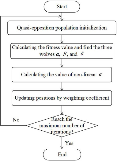
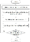
Figure 1: The flowchart of the QOGWO algorithm.

$${\overline{X}}_{\omega }(t+1)=\frac{\mathit{\text{f}}(\alpha ){\overline{P}}_{\alpha }(t)+\mathit{\text{f}}(\beta ){\overline{P}}_{\beta }(t)+\mathit{\text{f}}(\delta ){\overline{P}}_{\delta }(t)}{\mathit{\text{f}}(\alpha )+\mathit{\text{f}}(\beta )+\mathit{\text{f}}(\delta )},$$

(6)

where the weighting function $\mathit{\text{f}}(\cdot )$ is the fitness value of the individual.

After the improvement in Subsections A-C, the GWO algorithm is modified into the QOGWO version, whose flowchart is demonstrated in Fig. 1.

III. HYBRID ALGORITHM OF QOGWO AND GPR

In the QOGWO algorithm, each individual denotes a vector whose components are dimension parameters of the antenna and randomly valued within the ranges. Calculating the fitness value of each individual requires one full wave simulation. For complex antennas, the time cost may be unacceptable. For reducing the times of full wave simulations, the GPR model is introduced to predict the fitness values of individuals in this section.

In the GPR model, the mean function and the covariance function determine its prediction accuracy. The mean function often takes a value of 0. The suited kernel function serves as the covariance function [12]. For improving its performance, the hyperparameters of the kernel function are usually optimized by the conjugate gradient (CG) algorithm [10]. However, the CG algorithm has the shortcomings of over-dependence on the initial value, easily falling into local optimal solution, and poor convergence. As a remedy, the QOGWO algorithm is preferably chosen as the optimizer of hyperparameter due to its merits, shown in Section II A-C.

The QOGWO and the above improved GPR model are combined into the QOGWO-GPR algorithm. It consists of two steps. The first step is training the GPR prediction model, where the QOGWO is used to optimize the hyperparameters of the different kernel functions for obtaining the best-fitting model. The second step is optimizing individuals, i.e., sets of dimension parameters of antenna, where the QOGWO invokes the trained GPR model to calculate the fitness values of individuals. The process will be detailed in the simulation experiments below.

IV. EXAMPLES AND ANALYSIS

A stepped ultrawide-band monopole antenna [11] and a dual-band MIMO antenna for WLAN [14] are used to validate the hybrid QOGWO-GPR algorithm. The simulations are performed on a computer with Core i7-8700K CPU and 32 GB memory.

A. A stepped ultrawideband monopole antenna

A.1 Configuration of antenna

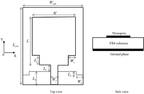
Figure 2 shows the configuration of the antenna. The middle layer is the dielectric substrate FR4 (${ϵ}_r$ = 4.5, $h$ = 1.6 mm). The top surface of the dielectric substrate is partially covered with a stepped monopole radiator patch, which is fed by 50 $\mathrm{\Omega }$ microstrip line. On the bottom surface is a corner-truncated ground plate. The stepped design of both layers is capable of decreasing the discontinuity of the structure at the antenna feed source and improving the impedance matching of the antenna [11]. The frequency $fre$ varies from 2 to 12 GHz.

Figure 2: Configuration of the stepped ultrawideband monopole antenna ($W_{sub}$ = 20 mm, $L_{sub}$ = 30 mm, $W$ = 16 mm, $L$ = 18 mm, $L_4$ = 5 mm).

For broadening the bandwidth of the antenna and improving its directivity by the QOGWO-GPR algorithm, the performance targets here are $S_{11}$ and $Gain$. Dimension parameters to be optimized and their ranges are listed in Table 1.

Table 1: Dimension parameters and their ranges of the antenna

Parameters	$L_1$	$W_1$	$L_2$	$W_2$	$L_3$
Ranges (mm)	4-8	2-5	0.5-3	5-8	1.5-2.5

A.2 Training GPR prediction model

Firstly, we use HFSS simulation to calculate $S_{11}$ and $Gain$ of the samples. Then, samples are put into the GPR model. In the GPR model, the vector $[L_1,W_1,L_2,W_2,L_3,fre]$ is the input variable, and $S_{11}$ and $Gain$ are the output values. For each dimension parameter, three values are sampled uniformly within the range, and 243 sets are yielded. The frequency step is 500 MHz, so there are 5103 input samples.

The input sample data is divided into two parts: 70% samples randomly chosen as the training set and 30% samples as the test set. Based on the two sets, the kernel function candidates such as RQ, SE and Matern functions are built for the GPR model [12]. Their hyperparameters are optimized by the QOGWO algorithm, where$N$ is set to 24 and $Max\mathrm{\_}iter$ set to 30.

To reduce the bias in experimental results caused by randomness, the above test is conducted 10 rounds for each kernel function. The performance of the GPR model resulted from the kernel function is assessed by the root mean square error (RMSE) [13] as

$$\mathit{\text{RMSE}}=\sum _{d=1}^D\sqrt{\frac{1}{n}\sum _{i=1}^n{\left(y_i^d-{\widehat{y}}_i^d\right)}^2},$$

(7)

where $n$ is the number of test samples data. $D$ is the dimensionality of the output sample. $y_i^d$ is the output sample value, and ${\widehat{y}}_i^d$ is the predicted output sample value by the GPR model. Obviously, the smaller the RMSE, the better the prediction.

Our simulation results show that the Matern kernel function (with hyperparameters $l=3.713$ and ${\sigma }_f^2=1.654$) can achieve the best training effect. Thus, it serves as the covariance function in the GPR model. The RMSE changes with iterations, as shown in Fig. 3.

Figure 3: RMSE changes with iterations.

A.3 Simulation of QOGWO-GPR algorithm

In the QOGWO-GPR algorithm, one individual denotes the vector $[L_1,W_1,L_2,W_2,L_3]$. $N$ is set to 100 and $Max\mathrm{\_}iter$ set to 500. The dimension parameters and the ranges are listed in Table 1. Once the initial population and the quasi-opposition counterpart are generated, a trained GPR model is invoked to predict $S_{11}$ and $Gain$ of each individual at arbitrary frequencies.

For achieving the multi-objective optimization, weighting $S_{11}$ and $Gain$ yields the fitness value as

$$\mathit{\text{fitness}}=\frac{w_1}{\mathit{\text{Num}}}\sum _{i=1}^{\mathit{\text{Num}}}\frac{{\mathrm{S}}_{11}(i)}{S_{\text{tol}}}+\frac{w_2}{\mathit{\text{Num}}}\sum _{i=1}^{\mathit{\text{Num}}}\frac{Gai{n}_{\text{tol}}}{\mathrm{Gain}(i)},$$

(8)

where Num is the number of frequency points. The weight coefficients $w_1$ and $w_2$ are set to 0.5.$S_{\text{tol}}$ and $Gai{n}_{\text{tol}}$ are the tolerance values of two optimization targets, taken as -10 dB and 3 dBi respectively.${\mathrm{S}}_{11}(i)$ is the return loss at the $i$th frequency point after pre-processing by

$${\mathrm{S}}_{11}(i)=\{\begin{array}{c}-12,S_{11}(i)<-12\hfill \\ S_{11}(i),S_{11}(i)\ge -12.\hfill \end{array}$$

(9)

$\mathrm{Gain}(i)$ is the gain at the $i$th frequency point after normalization by

$$\mathrm{Gain}(i)=\{\begin{array}{c}\mid Gain(i)\mid ,Gain(i)<-3\hfill \\ 3,Gain(i)\ge -3.\hfill \end{array}$$

(10)

Finally, the QOGWO algorithm iterates until the individual with the best fitness value (i.e., the optimal solution) is generated. The optimized parameters of the antenna are: $L_1$ = 4.4 mm, $W_1$ = 5 mm, $L_2$ = 1.16 mm, $W_2$ = 8 mm and $L_3$ = 2 mm.

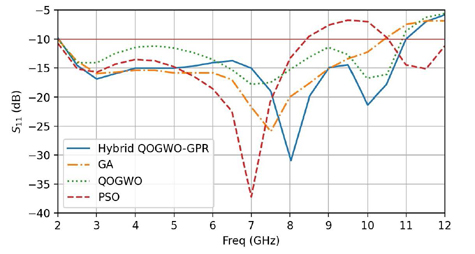
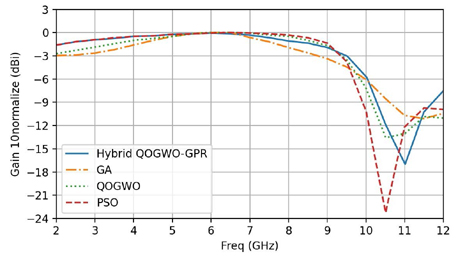
The hybrid QOGWO-GPR algorithm is compared with the genetic algorithm (GA), the particle swarm optimisation algorithm (PSO) and the QOGWO algorithm. In the later three algorithms, $N$ = 100, and $Max\mathrm{\_}iter$ = 100. The variance factor $p_m$ in the GA is set to 0.1 and the crossover probability factor $p_c$ set to 0.8. The learning factors $c_1$ and $c_2$ are set to 0.5, and the inertia factor $\omega$ set to 0.8 for the PSO. In these three algorithms, $S_{11}$ and $Gain$ for each individual are obtained from the HFSS software simulation, and the corresponding fitness value is generated via (8). When the maximum number of iterations is reached, the dimension parameters corresponding to the best fitness individual are put into the HFSS software for simulation. Figures 4 and 5 compare the results of $S_{11}$ and the normalized $Gain$ obtained from the different algorithms. Tables 2 and 3 list the statistical values, where Hybrid denotes the QOGWO-GPR, and ${\overline{S}}_{11}$ the average $S_{11}$.

Figure 4: Comparison of $S_{11}$ curves from different algorithms.

Figure 5: Comparison of normalized $Gain$ curves from different algorithms.

Table 2: Statistical values of impedance bandwidths from different algorithms

Algorithm	Bandwidth	${\overline{\mathit{S}}}_{\mathbf{11}}$
GA	107.56% (2 GHz-10.39 GHz)	-14.67 dB
PSO	82.31% (2 GHz-8.42 GHz)	-14.56 dB
QOGWO	113.84% (2 GHz-10.88 GHz)	-12.77 dB
Hybrid	113.97% (2.06 GHz-10.95 GHz)	-15.30 dB

Seen from the above figures and tables, the antenna optimized by the hybrid QOGWO-GPR algorithm has the best overall performance, and fully satisfies the design requirements. The one by the QOGWO algorithm has the second best overall performance, and the average $S_{11}$ is 2 dB higher than these by the GA and PSO algorithms.

Table 3: Statistical values of gains from different algorithms

Algorithm	-3dB Gain Bandwidth
GA	6.69 GHz (2.03 GHz-8.72 GHz)
PSO	7.31 GHz (2 GHz-9.31 GHz)
QOGWO	7.45 GHz (2 GHz-9.45 GHz)
Hybrid	7.53GHz (2 GHz-9.53 GHz)

In this example, the time cost of the hybrid QOGWO-GPR algorithm consists of three parts: generating the sample data, yielding the best-fitting GPR model, and optimizing the antenna size parameters. It takes a total of 7.47 hours. In the other three algorithms, the time cost of the individual updating position is negligible, and the time is mainly consumed by HFSS simulation for yielding the fitness values. It takes a total of 25.93 hours. The hybrid QOGWO-GPR algorithm takes about 28.8% of the time of the other three algorithms, respectively.

B. Dual-band MIMO antenna for WLAN

B.1 Configuration of antenna

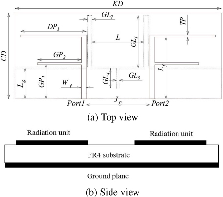
Figure 6 shows the configuration of the antenna [14]. It generates two separate resonant modes to cover 2.45 and 5 GHz WLAN bands. The middle layer is the dielectric substrate chosen as FR4 (${ϵ}_r$ = 4.4, $h$ = 0.8 mm). The antenna consists of two radiating units, which are the same and located symmetrically. The F-type antenna with two branches resonates at low frequency and high frequency, respectively. Two I-type floor branches and a floor gap act as an isolator.

In the QOGWO-GPR algorithm, the performance targets here are $S_{11}$ and $S_{21}$. The dimension parameters determining $S_{11}$ and $S_{21}$ are listed in Table 4. They are optimized by the QOGWO-GPR algorithm for broadening the bandwidth of the antenna and improving its isolation.

Figure 6: Configuration of the dual-band MIMO antenna for WLAN ($KD$ = 63 mm, $CD$ = 28 mm, $W_f$ = 1.4 mm, $L_f$ = 18 mm, $G{P}_1$ = 9 mm, $J_g$ = 18.5 mm, $L_g$ = 8.9 mm, $G{L}_2$ = 1.4 mm, $G{L}_4$ = 5.9 mm, $L$ = 15.1 mm).

Table 4: Dimension parameters and their ranges of the dual-band MIMO antenna

Parameters	$D{P}_1$	$G{L}_1$	$G{L}_3$
Ranges (mm)	17.37-21.23	13.86-16.94	0.5-0.9
Parameters	$LF$	$TP$	$G{P}_2$
Ranges (mm)	16.2-19.8	0.5-0.7	11.52-14.08

B.2 Training GPR prediction model

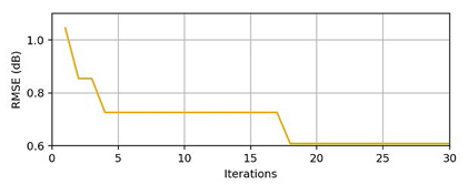
In the GPR model, $S_{11}$ and $S_{21}$ are the output values, and the vector $[D{P}_1,G{L}_1,G{L}_3,G{P}_2,LF,TP,fre]$ is the input variable. For each dimension parameter, three values are sampled uniformly within the range, and 729 sets are yielded. The frequencies are 2, 2.3, 2.45, 2.8, 4.4, 5, 5.3, and 5.9 GHz, so there are 5832 input samples. Then, putting samples into the GPR model, we optimize their hyperparameters by the QOGWO algorithm, where$N$ is set to 24 and $Max\mathrm{\_}iter$ set to 30. The GPR model simulation results show that the Rational Quadratic kernel function(with hyperparameters $l$ = 4.79, $\alpha$ = -0.76 and ${\sigma }_f^2$ = 0.06) can achieve the best training effect. Thus, it serves as the covariance function in the GPR model. The RMSE changes with iterations, as shown in Fig. 7.

Figure 7: RMSE changes with iterations.

B.3 Simulation of QOGWO-GPR algorithm

In the QOGWO-GPR algorithm, one individual denotes the vector $[D{P}_1,G{L}_1,G{L}_3,G{P}_2,LF,TP]$. $N$ is set to 30, and $Max\mathrm{\_}iter$ set to 50. The dimension parameters and the ranges are the same as those in Table 4. For achieving the multi-objectives optimization, weighting $S_{11}$ and $S_{21}$ yields the fitness value as

$$\mathit{\text{fitness}}=\frac{w_1}{\mathit{\text{Num}}}\sum _{i=1}^{\mathit{\text{Num}}}\frac{{\mathrm{S}}_{11}(i)}{S_{11\text{tol}}}+\frac{w_2}{\mathit{\text{Num}}}\sum _{i=1}^{\mathit{\text{Num}}}\frac{{\mathrm{S}}_{21}(i)}{S_{21\text{tol}}},$$

(11)

where Num is the number of frequency points. The weight coefficients $w_1$ and $w_2$ are set to 0.5 each.$S_{11\text{tol}}$ and $S_{21\text{tol}}$ are the tolerance values of two optimization targets, taken as -10 dB and -15 dB, respectively.${\mathrm{S}}_{11}(i)$ is the modified return loss at the $i$th frequency point after pre-processing by (9). ${\mathrm{S}}_{21}(i)$ is the modified isolation between two ports at the $i$th frequency point after normalization by

$${\mathrm{S}}_{21}(i)=\{\begin{array}{c}\hfill -15,S_{21}(i)<-15\hfill \\ \hfill S_{21}(i),S_{21}(i)\ge -15.\hfill \end{array}$$

(12)

Finally, the QOGWO algorithm iterates until the individual corresponding to the best fitness value (i.e., the optimal solution) is generated. The optimized parameters of the antenna are: $D{P}_1$ = 21.23 mm, $G{L}_1$ = 16.48 mm, $G{L}_3$ = 0.5 mm, $G{P}_2$ = 14.08 mm, $LF$ = 16.2 mm, and $TP$ = 0.5 mm. The hybrid QOGWO-GPR algorithm takes a total of 20.18 hours.

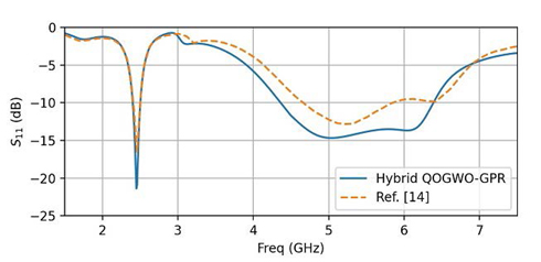
Figure 8: Comparison of $S_{11}$ curves between Ref. [14] and the hybrid algorithm.

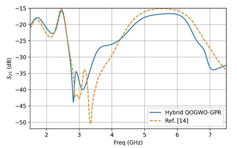
Figure 9: Comparison of $S_{21}$ curves between Ref. [14] and the hybrid algorithm.

The values are input into HFSS simulation, and the results are shown in Figs. 8 and 9. After optimization, two operation frequency bands are 2.40 GHz – 2.50 GHz and 4.36 GHz – 6.39 GHz, and the isolation of all operation frequency bands is less than -15 dB. In [14], the two bandwiths at 2.45 and 5 GHz are 36.7% and 23.8%, respectively. And these are 40.8% and 40.6%, respectively, in the hybrid QOGWO-GPR. Table 5 shows the comparison between the Ref. [14] and the hybrid algorithm.

Table 5: Comparison between Ref. [14] and the hybrid algorithm

	2.45GHz	5GHz
Ref. [14]	2.39 GHz-2.48 GHz	4.64 GHz-5.83 GHz
Hybrid	2.40 GHz-2.50 GHz	4.36 GHz-6.39 GHz

V. CONCLUSION

In this paper, the hybrid QOGWO-GPR algorithm is presented to improve the GWO algorithm in antenna optimization. It is prone to global optimality, high precision for complex problems and fast convergence rate at the later stage. It can also reduce the optimization time of the antenna. We have given two examples to validate the proposed algorithm in this work. At low time cost, for the stepped ultrawideband monopole antenna, the impedance bandwidth can reach 113.97% and the -3 dB gain bandwidth can reach 7.53 GHz; for the dual-band MIMO antenna for WLAN, the impedance bandwidths can reach 40.8% and 40.6% at 2.45 and 5 GHz, respectively, and the isolation of all operation frequency bands is less than -15 dB.

ACKNOWLEDGMENT

This work was supported in part by the NKRDP (2019YFB1803202) and the NSFC (62131008 and 62293492).

REFERENCES

[1] A. Nysaeter, “Two-way MIMO sparse array antenna optimization with NSGA-III,” 2020 IEEE Radar Conference (Radar-Conf20). IEEE, pp. 1-6, 2020.

[2] A. Singh, R. Mehra, and V. Pandey, “A hybrid approach for antenna optimization using cat swarm based genetic optimization,” Advanced Electromagnetics, vol. 7, no. 3, pp. 23-34, 2018.

[3] S. Mirjalili, S. M. Mirjalili, and A. Lewis, “Grey wolf optimizer,” Advances in Engineering Software, vol. 69, pp. 46-61, 2014.

[4] Y. Zhang, J. Li, and M. Zhang, “Motion key frame extraction based on grey wolf optimization algorithm,” MATEC Web of Conferences, vol. 232, no. 03032, pp. 1-5, 2018.

[5] C. Han, M. Chen, L. Pan, and X. Chen, “A community detection algorithm by utilizing grey wolf optimization,” 2017 9th International Conference on Modelling, Identifcation and Control (ICMIC), IEEE, pp. 567-572, 2017.

[6] H. Faris, I. Aljarah, M. A. Al-Betar, and S. Mirjalili, “Grey wolf optimizer: A review of recent variants and application,” Neural Computing and Applications, vol. 30, no. 2, pp. 413-435,2018.

[7] C.-F. Wang, K. Liu, and P.-P. Shen, “A novel genetic algorithm for global optimization,” Acta Mathematicae Applicatae Sinica, English Series, vol. 36, no. 2, pp. 482-491, 2020.

[8] L. Peng and Y. Wang, “Differential evolution using uniform-quasiopposition for initializing the population,” Information Technology Journal, vol. 9, no. 8, pp. 1629-1634, 2010.

[9] S. Rahnamayan, H. R. Tizhoosh, and M. M. Salama, “Quasi-oppositional differential evolution,” 2007 IEEE Congress on Evolutionary Computation, pp. 2229-2236, 2007.

[10] J. R. Shewchuk, “An introduction to the conjugate gradient, method without the agonizing pain,” Ph.D. dissertation, Carnegie-Mellon University, 1994.

[11] S. Sun, “Compact wideband microstrip antenna design based on improved genetic algorithm,” Ph.D. dissertation, Beijing University of Posts and Telecommunications, 2011.

[12] E. Schulz, M. Speekenbrink, and A. Krause, “A tutorial on gaussian process regression: Modelling, exploring, and exploiting functions,” Journal of Mathematical Psychology, vol. 85, pp. 1-16,2018.

[13] T. O. Hodson, “Root mean square error (RMSE) or mean absolute error (MAE): When to use them or not,” Geoscientifc Model Development Discussions, pp. 1-10, 2022.

[14] T. Ma, C. Du, and Z. Jiao, “Miniaturized dual-band MIMO antenna for WLAN,” Instrumentation Technology, pp. 7-10, 2019.

BIOGRAPHIES

Hao-Yun Zhu received the M.S. degree in computer technology in 2022 from Southeast University, Nanjing, China. During the graduate period, he majored in electromagnetic computation, and his research interest focuses on optimization algorithms for electromagnetic simulations.

Jia-Wei Qian received the B.S. degree in electronic and information engineering in 2020 from the Nanjing University of Posts and Telecommunications, Nanjing, China. He is currently working toward for the master’s degree in electronic and information engineering at Southeast University. His current research interest is full-wave algorithm in time domain and optimization algorithms.

Xiao-Hui Tang received the B.S. degree in electromagnetic fields and wireless technology in 2021 from the Nanjing University of Posts and Telecommunications, Nanjing, China, where she is currently working toward the master’s degree in electronic and information engineering at Southeast University. Her current research interest is optimization algorithms for antenna array.

Wei-Dong Li received the M.S. degree in mathematics and the Ph.D. degree in radio engineering from Southeast University, Nanjing, China, in 2003 and 2007, respectively.

He is currently an associate professor of School of Information Science and Engineering. From January 2008 to January 2009, he was a visiting scholar with the Technische Universität Darmstadt, Germany. His research interests include optimization of sparse antenna array, integral equation numerical modeling and fast algorithm, fast and accurate inter/extrapolation techniques, and DGTD in computational EM. He has authored or co-authored over 40 technical papers. He serves as reviewers for IEEE Transactions on Antennas and Propagation and IET Microwave, Antennas and Propagation.

ACES JOURNAL, Vol. 38, No. 9, 674–680
doi: 10.13052/2023.ACES.J.380906
© 2023 River Publishers

ABSTRACT

I. INTRODUCTION

II. IMPROVED GWO

A. Quasi-opposition population initialization

B. Non-linear convergence factor

C. Updating positions by weighting coefficients

III. HYBRID ALGORITHM OF QOGWO AND GPR

IV. EXAMPLES AND ANALYSIS

A. A stepped ultrawideband monopole antenna

A.1 Configuration of antenna

A.2 Training GPR prediction model

A.3 Simulation of QOGWO-GPR algorithm

B. Dual-band MIMO antenna for WLAN

B.1 Configuration of antenna

B.2 Training GPR prediction model

B.3 Simulation of QOGWO-GPR algorithm

V. CONCLUSION

ACKNOWLEDGMENT

REFERENCES

BIOGRAPHIES