Improved and Easy-to-implement HFSS-MATLAB Interface without VBA Scripts: An Insightful Application to the Numerical Design of Patch Antennas
Giacomo Giannetti
Department of Information Engineering
Università degli Studi di Firenze, Florence, Italy
giacomo.giannetti@unifi.it
Submitted On: April 6, 2023; Accepted On: July 3, 2023
ABSTRACT
An improved and easy-to-implement HFSS-MATLAB interface is presented. Because the interface is realized without the use of VBA scripts, it is easier to implement for beginners and practitioners. This advantage allows more dissemination of the code in the HFSS community. The interface is applied to the numerical design of a patch antenna, showing the capabilities it enables. Practical details about the implementation are provided, enabling the reader to implement the interface on their own.
Index Terms: application programming interface, HFSS, hierarchical optimization, MATLAB, patch antenna.
I. INTRODUCTION
Modern programs for computer-aided design (CAD) are extremely useful tools for the design of complex structures. However, they are difficult to manage when they have to be interfaced with other software or when complex operations are necessary [1, 2].
In order to manage complex operations involving CAD software in a straightforward way, it is of paramount importance to be able to interface CAD software with a numeric computing environment (NCE). In the following, we refer to HFSS [3] and MATLAB [4].
The development of an HFSS-MATLAB interface is not new. It is described in [5, 6, 7, 8], and a library for the interface between MATLAB and HFSS is available online [9]. In [1, 2], FEKO [10] is interfaced with MATLAB. Python has also been used recently to launch EM simulators [11, 12]. However, the mentioned works use the Visual Basic for Applications (VBA) scripting language to interface HFSS and MATLAB. VBA scripts require large libraries, since each feature in the HFSS model requires a specific command with a specific syntax. Then, even if HFSS commands can be recorded to a script exploiting a useful feature of HFSS [6], writing a script is a slow and tedious task, especially for beginners. Another possibility to interface HFSS and MATLAB is to call the latter during the execution of the former. However, this interface is much less flexible than the one in which MATLAB drives HFSS. Not to be forgotten, students and experienced designers can feel pain when they have to learn a further programming language [13].
This paper presents and describes an improved and easy-to-implement HFSS-MATLAB interface that makes no use of VBA scripts. To achieve this goal, variables are updated in the ASCII file describing the HFSS model to simulate. Practical details are provided for the implementation of the application programming interface (API). Moreover, for easier reproducibility of the API, working examples are also available at [14]. Thanks to the API, there is no need to learn VBA to script HFSS. This CAD is then treated like a black box that returns the output of a simulation once it is called from MATLAB. The working principles of the API are presented in a practical example: the numerical design of a patch antenna resonating at GHz.
II. DESIGN EXAMPLE
The example considered for illustrating the proposed interface is the numerical design of a rectangular patch antenna working at GHz. The substrate of the antenna is characterized by a height of mm, a metallization thickness of mm, and a relative dielectric constant of . The technical drawing of the proposed antenna is depicted in Fig. 1. The patch is characterized by a width and a length . The feed is a transformer whose length is . To have more degrees of freedom, the transformer has a trapezoidal shape whose bases are and , where mm, the width of the microstrip with a characteristic impedance. The distance between the patch and the sides of the substrate is mm and the length of the microstrip is mm. In the following, only parameters , , , , and are variable, the others being constants.
Figure 1: Technical drawing of the patch antenna.
Table 1: Variable history (dimensions in millimeters, abbreviation a.a. stands for as above)
| Variables | |||||
| L | W | a | b | c | |
| Min | 46 | 57 | 26 | 1.500 | 1.500 |
| Max | 50 | 61 | 32 | 2.370 | 2.370 |
| Anal. | 49.830 | 59.290 | 28.510 | 2.070 | 2.070 |
| Opt. (i) | 48.472 | a.a. | a.a. | a.a. | a.a. |
| Opt. (ii) | a.a. | 59.225 | 28.440 | 2.014 | 1.999 |
An analytical design procedure for rectangular patch antennas is possible [15], and the values of the geometrical parameters for this design are listed in Table 1. However, once the geometrical values from the analytical design are simulated, the antenna results do not match them at the desired working frequency, as shown in Fig. 2. The resonant frequency (the frequency at which the minimum of the return loss occurs), the minimum of the return loss and the return loss at GHz, , are gathered in Table 2.
To have an antenna working at the desired frequency, an optimization is performed. Since the magnitude of the reflection coefficient is not a smooth function of the geometrical parameters [16], it is not wise to consider a unique goal for the optimization of the return loss. Then, the problem is tackled by means of a hierarchical optimization with these two goals:
| (1a) | |||
| (1b) |
where stands for minimize. The reasons behind the definitions of these two optimizations derive from the theory of the problem. Indeed, it is known from theory [15] that a) the resonant frequency depends primarily on the patch length, and b) matching depends primarily on the feed dimensions and patch width. Then the two optimizations of the hierarchical optimization are (1a) for point a and (1b) for point b. Note that while improving matching in (1b) we do not care about the resonant frequency of the antenna, assuming that it does not change remarkably. However, if the change in the resonant frequency after solving (1b) is remarkable, then optimization (1a) can be repeated to re-center the resonant frequency at the desired value.
For the above optimizations, the MATLAB optimization functions are fminbnd for (1a), and fmincon for (1b). Function fminbnd is especially useful for minimization problems with a single variable. As starting point for the hierarchical optimization, the analytical design is considered. The minimum and maximum values for the variables being optimized are listed in Table 1.
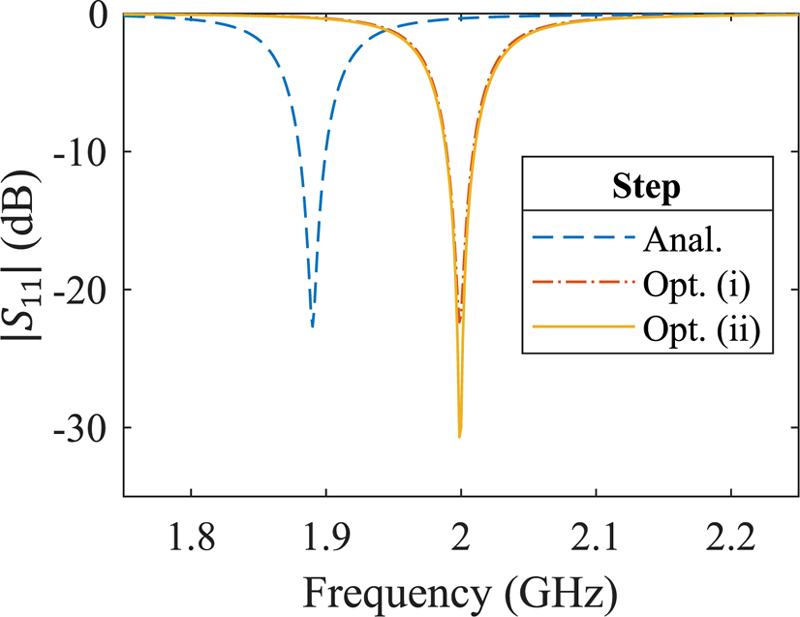
Figure 2: Magnitude of for the patch antenna during the different steps of the design.
Table 2: Result summary
| Step | (GHz) | (dB) | (dB) |
|---|---|---|---|
| Anal. | 1.890 | -22.68 | -0.35 |
| Opt. (i) | 1.999 | -22.37 | -21.83 |
| Opt. (ii) | 1.999 | -30.70 | -29.99 |
III. DESCRIPTION OF THE API
In the following, the filenames indicated in Table 3 are considered. Obviously, only the file extension must be the one indicated while the filename could be different, provided that all occurrences change accordingly.
Table 3: Files for the API
| Filename | Description |
|---|---|
| HFSS_API.m | MATLAB script for the interface |
| base.aedt | Model to simulate |
| base.txt | Model with signposts |
| modified.aedt | Model with updated variables |
| ExportToFile.py | Python script for data extraction |
| res.csv | Exported results |
The MATLAB commands are in HFSS_API.m. The HFSS model to simulate is base.aedt, while base.txt is the same as base.aedt, but with the variables substituted by univocal signposts. The file modified.aedt is the HFSS model to simulate with updated variables. Eventually, ExportToFile.py is the Python script for the export of the results and res.csv the exported results.
The flow chart for the proposed API is presented in Fig. 3. The proposed API is made of steps to be done once, called Preliminary steps, and steps that have to be done before each simulation, called Steps to be repeated. The preliminary steps are done manually by the designer, while the API automatically performs the others. Furthermore, the blocks with rounded corners refer to the steps performed in MATLAB, while those without rounded corners to those of the API.
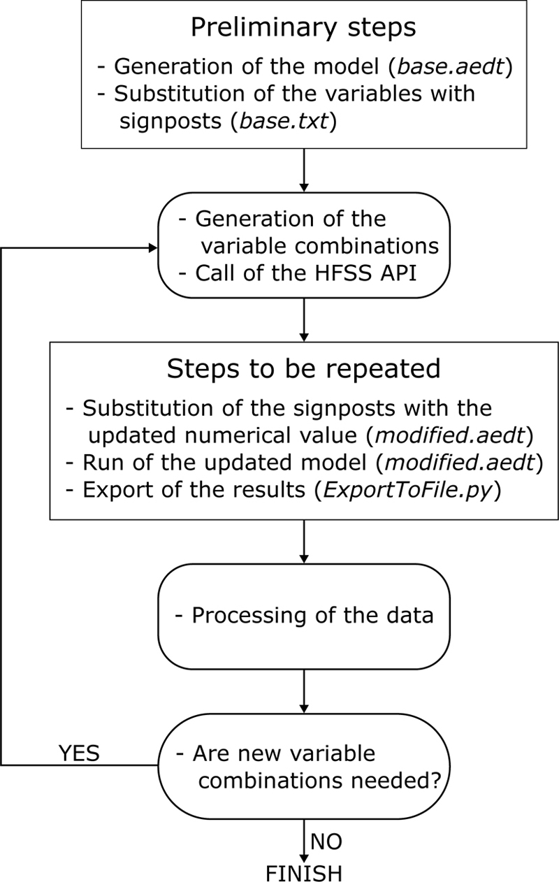
Figure 3: Flow chart of the proposed API. The rectangles with rounded corners refer to the steps performed in MATLAB, while those without rounded corners relate to the proposed API.
A. Preliminary steps
The preliminary steps are:
∙ build the model in HFSS and save it as base.aedt;
∙ copy the previous file and open it as a text file. Substitute the numerical values of the variables to be varied with unique character combinations (‘signposts’, one for each variable), and save the file as base.txt;
∙ generate the file ExportToFile.py to export the results of the simulation.
Since all setups are run by the command used to execute the simulations, the designer, while preparing the HFSS model, should follow these directions: a) insert only one design, called Design in the following; b) insert only the required setups.
Here is the part of file base.txt defining the variables of the design: the signposts inserted to substitute for the variables are shown in bold:
$begin ‘Properties’
VariableProp(‘A’, ‘UD’, ‘’, ‘1A1Amm’)
VariableProp(‘B’, ‘UD’, ‘’, ‘1B1Bmm’)
VariableProp(‘a’, ‘UD’, ‘’, ‘2A2Amm’)
VariableProp(‘b’, ‘UD’, ‘’, ‘2B2Bmm’)
VariableProp(‘c’, ‘UD’, ‘’, ‘2C2Cmm’)
VariableProp(‘ts’, ‘UD’, ‘’, ‘1.6mm’)
VariableProp(‘tc’, ‘UD’, ‘’, ‘0.035mm’)
VariableProp(‘Le’, ‘UD’, ‘’, ‘8mm’)
VariableProp(‘Lm’, ‘UD’, ‘’, ‘10mm’)
VariableProp(‘M’, ‘UD’, ‘’, ‘4.942869528525mm’)
$end ‘Properties’.
Here is the Python file ExportToFile.py to export the results of the simulation:
oDesktop.RestoreWindow()
oProject = oDesktop.SetActiveProject(“Modified”)
oDesign = oProject.SetActiveDesign(“Design”)
oModule = oDesign.GetModule(“ReportSetup”)
oModule.UpdateReports([“S11mag”])
oModule.ExportToFile(“S11mag”, “res.csv”),
where Design is the name of the design in modified.aedt and S11mag is the name of the report displaying the results. The file ExportToFile.py could even be generated automatically in MATLAB.
B. Steps to be repeated
The steps to be repeated for each parameter combination request by the MATLAB script are:
∙ read file base.txt containing signposts, substitute each signpost with the numerical values indicated by the MATLAB script, and save the new file as modified.aedt;
∙ run file modified.aedt to simulate the model;
∙ run file ExportToFile.py to export results;
∙ read the results exported in file res.csv.
While substituting the numerical values with signposts, the designer must be aware of the right correspondence between the substituted variables and the actual variables in the model. Therefore, it is helpful to note a correspondence table while inserting the signposts. For example, after having substituted the numerical variables, the file modified.aedt appears as
$begin ‘Properties’
VariableProp(‘L’, ‘UD’, ‘’, ‘48.47213595500mm’)
VariableProp(‘W’, ‘UD’, ‘’, ‘59.22459629087mm’)
VariableProp(‘a’, ‘UD’, ‘’, ‘28.44027653740mm’)
VariableProp(‘b’, ‘UD’, ‘’, ‘2.013573376324mm’)
VariableProp(‘c’, ‘UD’, ‘’, ‘1.999106250004mm’)
VariableProp(‘ts’, ‘UD’, ‘’, ‘1.6mm’)
VariableProp(‘tc’, ‘UD’, ‘’, ‘0.035mm’)
VariableProp(‘Le’, ‘UD’, ‘’, ‘8mm’)
VariableProp(‘Lm’, ‘UD’, ‘’, ‘10mm’)
VariableProp(‘M’, ‘UD’, ‘’, ‘4.942869528525mm’)
$end ‘Properties’.
The MATLAB command that executes a string in the command window is system(StringToExecute). The string for simulating the HFSS model is
“PathExe\ansysedt.exe” /Ng /BatchSolve
“Path\modified.aedt”,
while the string for exporting the results is
“PathExe\ansysedt.exe” /Ng /BatchExtract
“Path\ExportToFile.py” “Path\modified.aedt”,
where ansysedt.exe is the executable for HFSS, PathExe is the folder where the executable file ansysedt.exe is stored, /Ng is the setting enabling the non-graphical mode, and Path is the folder where the files listed in Table 3 are saved.
IV. RESULTS
After running optimizations (1a) and (1b), the results for the reflection coefficient are presented in Fig. 2, and the values of the variables are listed in Table 1. Data summarizing the optimization are gathered in Table 2.
We note that it is sufficient to operate only on the length of the patch to have it resonating at the desired frequency. Additionally, optimization (1b) on the other parameters successfully improves matching without affecting the resonant frequency. Eventually, the first optimization requires only 2 function evaluations while the second requires 13, thus proving the effectiveness of the hierarchical optimization over indiscriminate global optimization algorithms like genetic ones [17, 18].
V. CONCLUSIONS
A useful interface between a CAD software, HFSS, and a software for technical computing, MATLAB, is outlined. Unlike other approaches performing the same task, the proposed one makes no use of VBA scripts to drive HFSS, hence being easier to implement and allowing the execution of simulations in non-graphical mode.
A glance into the interesting features enabled by this interface is provided by means of an example: the tuning of a resonant patch antenna. Despite this rather simple problem, it shows how the proposed API interface can realize complex procedures. Indeed, without the API, the designer would launch the different optimizations manually, with a high risk of errors and the need to keep up with the execution. On the contrary, with the proposed API, all steps of the hierarchical optimization can be handled automatically in MATLAB with much more flexibility.
Even though this interface is developed to drive HFSS, its working principles are of general validity and can be adapted to drive other simulators or software. For instance, the author applied the proposed method to drive GPT [19], a code for particle simulations.
Here what we learned from this lesson. Firstly, for the happiness of many, there is no need to learn VBA. Secondly, despite the computation capabilities we are experiencing nowadays, a good knowledge of the theory behind what we are studying is fundamental. The analyzed example shows how a hierarchical optimization approach can tune a patch antenna with only few 3D full-wave simulations.
ACKNOWLEDGEMENTS
The author thanks Prof. Pelosi for having prompted him to publish a single-author paper and to Eng. Maddio for having verified the proposed interface with more complex designs. The author is grateful also to Prof. Selleri and Eng. Righini for hints on how to run HFSS simulations from the command window. All acknowledged persons are from the University of Florence.
REFERENCES
[1] R. L. Haupt, “Using MATLAB to control commercial computational electromagnetics software,” Applied Computational Electromagnetics Society (ACES) Journal, vol. 23, no. 1, pp. 98-103, 2008.
[2] A. Farahbakhsh, D. Zarifi, and A. Abdolali, “Using MATLAB to model inhomogeneous media in commercial computational electromagnetics software,” Applied Computational Electromagnetics Society (ACES) Journal, vol. 30, no. 9, pp. 1003-1007, 2015.
[3] “Ansys — Engineering Simulation Software,” [Online] Available: https://www.ansys.com/, 2022.
[4] “MathWorks,” [Online] Available: https://www.mathworks.com/, 2022.
[5] Q. Tan, K. Fan, W. Yang, and G. Luo, “Low sidelobe series-fed patch planar array with AMC structure to suppress parasitic radiation,” Remote Sensing, vol. 14, no. 15, p. 3597, 2022.
[6] I. Bouchachi, “Microstrip antenna synthesis using an application programming interface,” Journal of Mechanics of Continua and Mathematical Sciences, vol. spl1, no. 4, 2019.
[7] J. B. Romdhane Hajri, D. Inserra, W. Gu, W. Hu, Y. Huang, J. Li, and G. Wen, “Fast and automatic RF design based on MATLAB-HFSS control applied on magnetic absorber with metasurface,” in 2019 Photonics and Electromagnetics Research Symposium - Fall, PIERS - Fall 2019 - Proceedings, 2019.
[8] X. Yuan, Z. Li, D. Rodrigo, H. S. Mopidevi, O. Kaynar, L. Jofre, and B. A. Cetiner, “A parasitic layer-based reconfigurable antenna design by multi-objective optimization,” IEEE Transactions on Antennas and Propagation, vol. 60, no. 6, 2012.
[9] V. Ramasami, “HFSS-API,” [Online] Available: https://github.com/yuip/hfss-api, 2020.
[10] “FEKO,” [Online] Available: https://www.altair.com/feko, 2023
[11] C. Fang, S. Xinyang, and X. Zeng, “Using Python to launch electromagnetic scattering simulation with FEKO,” in 2021 13th International Symposium on Antennas, Propagation and EM Theory (ISAPE), pp. 1-3, IEEE, 2021.
[12] R. J. Sánchez-Mesa, D. M. Cortés-Hernández, J. E. Rayas-Sánchez, Z. Brito-Brito, and L. De La Mora-Hernández, ‘‘EM parametric study of length matching elements exploiting an ANSYS HFSS MATLAB-Python driver,” in 2018 IEEE MTT-S Latin America Microwave Conference, LAMC 2018 - Proceedings, 2018.
[13] N. Shrestha, C. Botta, T. Barik, and C. Parnin, “Here we go again: Why is it difficult for developers to learn another programming language?” in Proceedings of the ACM/IEEE 42nd International Conference on Software Engineering, pp. 691-701, 2020.
[14] G. Giannetti, “Gianne97/HFSS-MATLAB-API -without-VBA-scripts: HFSS-MATLAB API without VBA scripts - publication,” [Online] Available: https://doi.org/10.5281/zenodo.8068428, 2023.
[15] C. A. Balanis, Antenna Theory: Analysis and Design, Fourth Edition, John Wiley & Sons, 2016.
[16] S. Selleri, S. Manetti, and G. Pelosi, “Neural network applications in microwave device design,” International Journal of RF and Microwave Computer-Aided Engineering, vol. 12, no. 1, 2002.
[17] D. Goldberg, Genetic Algorithms in Search, Optimization, and Machine Learning, Addison Wesley Series in Artificial Intelligence, Addison-Wesley, 1989.
[18] L. Tarricone, “A genetic approach for the efficient numerical analysis of microwave circuits,” Applied Computational Electromagnetics Society (ACES) Journal, pp. 87-93, 2000.
[19] “GPT,” [Online] Available: https://www.pulsar.nl/gpt/, 2023.
BIOGRAPHIES

Giacomo Giannetti (ACES Student Member and IEEE Graduate Student Member) received the B.Sc. degree (cum laude) in electronic and telecommunications engineering from the University of Florence, Florence, Italy, in 2019, and the M.Sc. degree (cum laude) in electronic engineering from the Sapienza University of Rome, Rome, Italy, in 2021, with award as excellent graduate. He is currently working toward a Ph.D. degree in electromagnetism with the University of Florence. He spent a period as a student with the Technical University of Vienna, Vienna, Austria, and the National Laboratory of Frascati, Rome, Italy and a period as a Research Guest with Kiel University, Kiel, Germany. His research interests include microwave devices and computational electromagnetics.
ACES JOURNAL, Vol. 38, No. 6, 377–381
doi: 10.13052/2023.ACES.J.380601
© 2023 River Publishers