A 3-D Global FDTD Courant-limit Model of the Earth for Long-time-span and High-altitude Applications

Yisong Zhang¹, Dallin R. Smith², and Jamesina J. Simpson¹

¹Department of Electrical and Computer Engineering, University of Utah, Salt Lake City, UT, USA
yisong.zhang.ee@gmail.com, jamesina.simpson@utah.edu

²Air Force Research Labs, Albuquerque, NM, USA
dallinsmith9@gmail.com

Submitted On: May 2, 2023; Accepted On: February 6, 2024

ABSTRACT

A new global 3-D finite-difference time-domain (FDTD) model is introduced to simulate electromagnetic wave propagation around the Earth, including the lithosphere, oceans, atmosphere, and ionosphere regions. This model has several advantages over existing global models, which include grids that follow lines of latitude and longitude and geodesic grids comprised of hexagons and pentagons. The advantages of the new model include: (1) it may be run at the Courant-Friedrichs-Lewy (CFL) time step (as a result, it is termed the Courant-limit model); (2) subgrids may be added to specific regions of the model as needed in a straight-forward manner; and (3) the grid cells do not become infinitely larger as the grid is extended higher in altitude. As a result, this model is a better candidate than the others for investigating electromagnetic phenomena over long time spans of interest and for investigating atmosphere-ionosphere-magnetosphere coupling. The new model is first described and then validated by comparing results for extremely low frequency (ELF) propagation attenuation with corresponding analytical and measurement results reported in the literature.

Index Terms: ELF, electromagnetic wave propagation, FDTD, global propagation, long-time and high-altitude simulations, scattering.

I. INTRODUCTION

The Earth-ionosphere waveguide is defined as the spherical cavity between the Earth’s surface and the bottom side of the ionosphere [1]. Within this waveguide, ultra-low frequency (ULF: $<$ 3 Hz) and extremely low frequency (ELF: 3 Hz–3 kHz) electromagnetic waves are capable of propagating globally as quasi-transverse electromagnetic (TEM) waves that experience very little attenuation. TEM and higher-order waveguide modes can also propagate globally in the Earth-ionosphere waveguide at frequencies ranging from the upper ELF band to very low frequencies (VLF: 3-30 kHz) [2] and even high frequencies (HF: 3–30 MHz) [3]. The propagation of electromagnetic waves in the Earth-ionosphere waveguide has been of interest for a wide variety of applications, including communications (e.g. [4]), geolocation and communications with submarines (e.g. [5]), studying lightning and sprites (e.g. [6, 7]), and remote sensing (e.g. [8]).

Two generations of 3-D global finite-difference time-domain (FDTD) models [9] of electromagnetic wave propagation in the Earth-ionosphere waveguide have been generated over the years: (1) latitude-longitude models (e.g. [10, 11]) and (2) geodesic models (e.g. [12]). Both generations of models have been used for a variety of applications (e.g. [13]), including Schumann resonances, hypothetical earthquake precursors, remote-sensing of ionospheric anomalies, space weather hazards to electric power grids, and remote sensing of oil fields.

In order to model beyond the Earth-ionosphere waveguide and to also pursue applications beyond those listed above, a new generation of global FDTD models is required. The reasons are three-fold:

(1) Both the latitude-longitude and geodesic grid cell arrangements require a time step increment that is smaller than the Courant-Friedrichs-Lewy (CFL) limit [9]. In the case of the latitude-longitude grid, this is due to the polar regions and the merging of cells [11]. For the case of the geodesic grid, the reduced time step is due to the reduction in the grid cell dimensions as any of the smaller 12 pentagons are approached (there are 12 pentagons in the model, regardless of the grid resolution) [12]. As a result of the reduced time step increment of these grid arrangements, many simulations of interest are challenging, if not infeasible, even using today’s supercomputing capabilities. An example scenario wherein a large number of time steps is required includes the generation of geomagnetically-induced currents (GICs) during geomagnetic storms. GICs are capable of causing blackouts to electric power grids. These storms can last days at a time, although the evolution of the storm over time spans of 30 minutes to two hours is often of most interest [14, 15]. Another example includes the global propagation of VLF to HF waves. It would take a large number of time steps for a wave to propagate around the entire Earth at the required grid resolution for VLF and HF waves. We note that the alternating direction implicit (ADI) FDTD approach [16–18] was used to generate a global FDTD model of the Earth-ionosphere waveguide [19]. However, that model was found to exhibit a late time instability, which limited the model’s utility, particularly for long time spans of interest.

(2) Adding efficient and stable subgrids to FDTD models continues to be a challenge. Many approaches have been proposed over the years, but an approach that is accurate and efficient for a wide variety of scenarios and for long time spans has not been established. Both the latitude-longitude grid and geodesic grids have the added complexity that the subgrids would have non-uniform cell sizes and domain edges. Further, the strategy for adding a subgrid to the geodesic model would need to change depending on whether the subgrid includes a pentagon or not.

(3) Both the latitude-longitude and geodesic grid cell arrangements are comprised of grid cells that become larger in the horizontal (East-West and North-South) directions as the grid is extended to higher altitudes. This becomes an issue for applications in which electromagnetic waves may couple into and propagate through the ionosphere and even into the magnetosphere (e.g. [20]). It is also an issue when studying the effects of space weather since the sources of electromagnetic waves (i.e., disturbed currents) occur throughout the ionosphere and magnetosphere regions [21].

In this paper, a new “global Courant-limit” FDTD model is presented that does not suffer from the above issues because all of the grid cells in the grid are Cartesian-based and identical. This allows the model to be run at the Courant limit, which is advantageous for long time spans. Furthermore, since all of the cells are uniform, the cells do not increase in size with increasing altitude. Finally, if at any point any subgrids are added to the model, the standard approach for regular Cartesian FDTD models may be utilized.

One disadvantage of the global Courant-limit model is that material interfaces, such as the Earth’s surface, are stair-cased. However, the staircasing is minimal because the grid resolution (5 km in this paper) is small compared to the radius of the Earth ( $\sim$ 6.4 Mm). Further, the staircasing reduces with increasing grid resolution, the surface of the Earth, in reality, is already not completely smooth, and techniques exist that may be used to mitigate the impact of staircasing as needed [22, 23].

The next section includes a description of the global Courant-limit model. Section III then provides details of the validation of the model. Section IV concludes the paper.

II. METHODOLOGY

A. Global Courant-limit model description

An example two-dimensional (2-D) slice of a low-resolution version of the three-dimensional (3-D) global Courant-limit model is shown in Fig. 1 (a). A higher-resolution 3-D view of the grid is shown in Fig. 1 (b). Although the grid is uniformly comprised of regular cubic grid cells, there are special considerations for the model, such as how to efficiently store the grid in computer memory, how to best center the grid, and how to assign boundary conditions and varying material parameters.

In the first part of the code (Part A), the grid is generated, and all of the updating coefficients are computed. The second part of the code (Part B) includes the time-stepping loop and any output from the model.

In Part A, the altitude range of the grid and the resolution of the cells are first defined. Thereafter, any Cartesian cells that are positioned within the altitude range of the model are assigned positive integer grid cell numbers. In the example slice of the grid shown in Fig. 1 (a), there are 28 total cells to be included in the model. The cells are positioned such that there are electric fields radiating outwards from the center of the Earth, as shown in Fig. 1 (a) (the center of the Earth is unlikely to be included in the model, so the electric field vectors shown at the center of the Earth are for illustrative purposes only). This field arrangement is optimal for dealing with the boundary conditions at the surface of the Earth. That is, using this arrangement the interface between the conductive lithosphere and the atmosphere is spherically symmetric, and it is comprised of a continuous string of tangential electric field components.

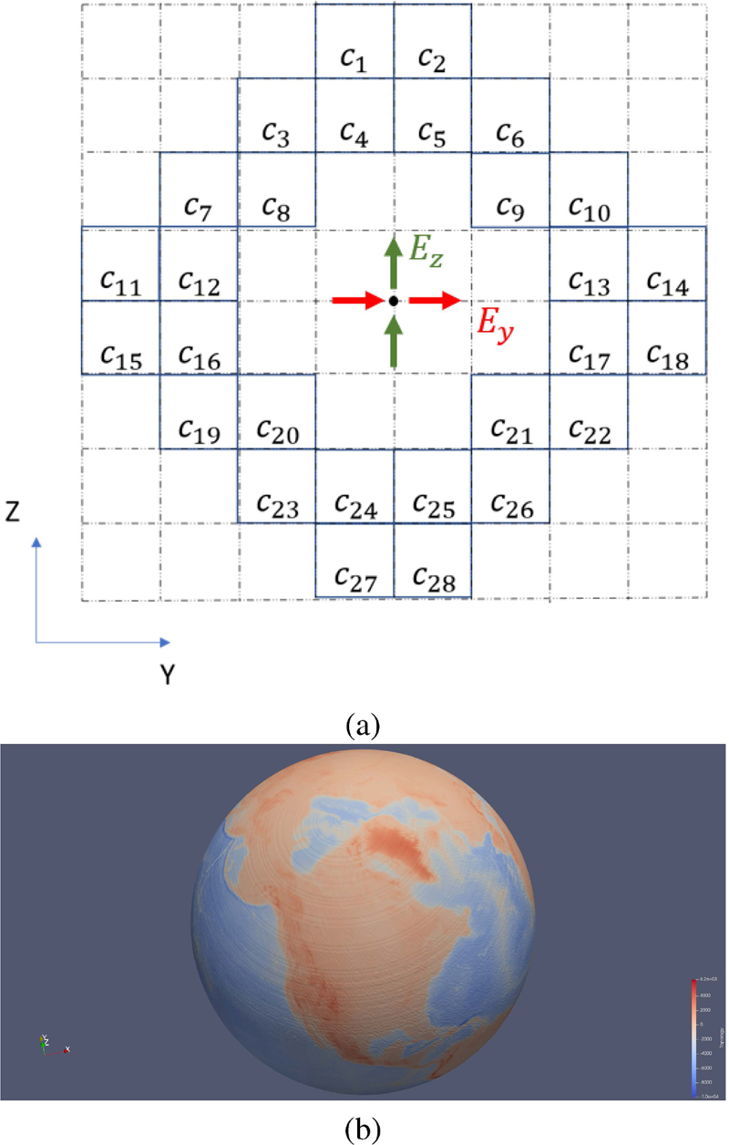
Figure 1: (a) Example 2-D slice of the 3-D grid cells along the prime meridian for the global Courant-limit model at a very low spatial resolution. Each cell (“c”) included in the model is labeled c $_{n}$ , where n represents the cell number. The arrows represent electric fields oriented radially from the center of the Earth, which is indicated by a black dot. (b) Illustration of the outer layer of the 3-D FDTD grid at a resolution of $5 \times 5 \times 5$ km with the Earth’s topography superimposed. Staircasing is minimal due to the size of the Earth, although this is difficult to fully visualize in an image of so many cells.

When generating the grid, there are two primary challenges. One of the biggest challenges is to ensure that there are not too many “ghost” cells (this was also true for the previous latitude-longitude model). Ghost cells take up memory but are not used in the time-stepping loop. The second challenge is to ensure that each processor is assigned the same number of grid cells such that the time-stepping loop is efficient. To address both of these issues, the field components in the global Courant-limit model are stored in 1-D arrays instead of 3-D matrices. This allows us to assign the same number of cells to each processor and prevents any ghost cells from being included. An effort is made to assign neighboring grid cells to the same processor to limit the number of communications required between processors (this is described further in Section IIB).

In order to implement a source or to record field values at specific locations, a weighted average approach is used on neighboring field components. This approach was also used in the latitude-longitude and geodesic grids. Special care must be taken across the air-lithosphere boundary (i.e., if a field observation in the atmosphere is desired, then only field values above the Earth’s surface should be utilized in the weighted average calculation).

Finally, for the second part of the code (Part B), the global Courant-limit model uses the same update equations in the time-stepping loop as found in regular Cartesian FDTD models [9]. The main difference is that the update equations use cell numbers in order to locate the neighboring cells since the data is stored in 1-D arrays instead of 3-D matrices. The updating coefficients and information about neighboring field components are all determined and stored in memory during the first part of the code (Part A) before time-stepping begins.

B. Parallelization of the grid

Message passing interface (MPI) is used to communicate between processors. In general, MPI communications are slow relative to the types of computations performed by each processor during the time-stepping loop. As a result, the goal when parallelizing the model is to minimize the amount of information that must be passed between processors using MPI. This is accomplished by assigning neighboring grid cells to the same processor as much as possible.

There are several methodologies that could be used to equally divide the cells onto different processors. One approach, which we followed, is to divide the grid first using a specific number of lines of longitude (with the number depending on how many processors will be used for the simulation). Thereafter, the grid is divided along the lines of latitude in a manner that assigns each processor the same volume of space. If a further division of the grid is needed, the volume of space may also be divided in the radial direction so that additional processors may be employed.

III. VALIDATION

The global Courant-limit model is validated by comparing the predicted ELF propagation attenuation with the data reported in [24]. As for the validation performed for the latitude-longitude model [25], the altitude range is set to be from -100 to +100 km, and the daytime exponential conductivity profile from [26] is used globally. Initially, the ground is considered to be a homogeneous perfect electric conductor (PEC) in order to test the model for spherical symmetry. The global Courant-limit model is run at a resolution of 5 $\times$ 5 $\times$ 5 km (rather than the 40 $\times$ 40 $\times$ 5 km resolution used in the latitude-longitude model of [11]). This grid resolution is chosen to match the 5-km resolution used in the radial direction of the latitude-longitude model.

The source is a radial, 5-km-long current pulse having a Gaussian time-waveform with a 1/e full-width of $1.44 m s$ . This current pulse is located just above the Earth’s surface on the equator and at the prime meridian. To ensure a smooth onset of the excitation, the temporal center of this pulse is $2.88 m s$ .

The radial electric field is sampled along the surface of the Earth in order to study its propagation characteristics. A few steps are required in order to obtain this data. Due to the staggering of the electric field components in the FDTD model, spatial averaging is first applied to the x-, y-, and z-electric field components in order to obtain the corresponding co-located values of these components at the specific observation points of interest. Specifically, up to eight electric fields closest to the observation point of interest are employed and averaged using an inverse-distance weighting (IDW) approach [27]. Once these co-located Cartesian components are obtained, they are converted to spherical coordinates in order to obtain the radial electric field.

A snapshot of the radial electric fields along the surface of the Earth is plotted in Fig. 2 after the pulse has propagated around the world and is in the process of converging at the antipode. The snapshot is obtained by recording the field values at 720x360 locations on the longitude-latitude grid. The black circles superimposed on the figure illustrate the model’s spherical symmetry very well.

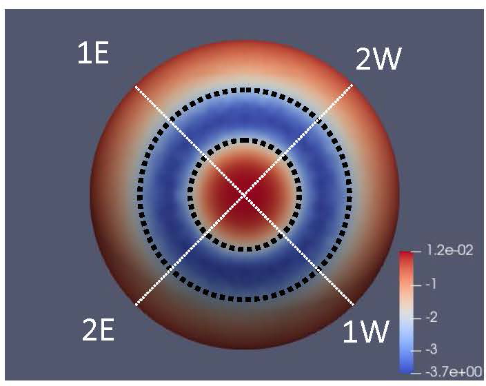
Figure 2: Visualization of the radial electric field projected onto the surface of the Earth-sphere after the pulse has propagated around the entire Earth and is converging at the antipode. The units for the electric field are $μ V / m$ . The spherical symmetry in the region of the antipode is apparent from the black dashed circles superimposed on the image.

The radial electric field is also recorded vs. time at several observation points along four different propagation paths between the source and its antipode. Point A along each propagation path corresponds to 1/4 of the distance to the antipode. Point B is 3/8 $^{t h}$ , Point C is 1/2, and Point D is 3/4 of the distance to the antipode. The orientations of these propagation paths are shown in Fig. 2 by the white dashed lines. Note that in 3-D, each of these propagation paths includes wave propagation along a variety of directions across the Cartesian-based grid cells.

Figure 3 shows the time waveforms of the FDTD-calculated radial electric fields at the A, B, C, and D observation points of all four propagation paths. Since the waveforms at each distance overlap, this plot also demonstrates the spherical symmetry of the model.

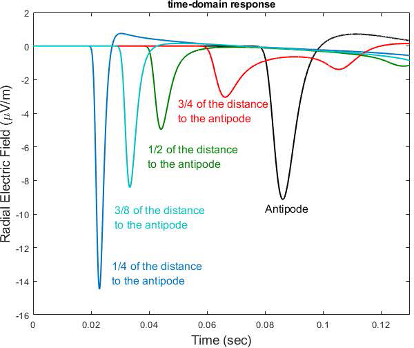
Figure 3: The FDTD-calculated time-domain response of the radial electric field along the four white dashed propagation paths shown in Fig. 2. The radial electric fields at observation points to the East of the source (along paths 1E and 2E) are labeled as solid lines, and the fields at points to the West of the source (along paths 1W and 2W) are labeled as dashed lines. All of the lines at each distance overlap, which indicates the global Courant-limit model’s spherical symmetrical.

Next, the topographic and bathymetric data from NOAA-NGDC is imported into the model, and lithosphere conductivities are assigned depending on whether a grid cell is located directly below an ocean or within a continent. A daytime profile is used globally as for the propagation attenuation study presented in [11].

Figure 4 compares the FDTD-calculated ELF propagation attenuation as calculated from the global Courant-limit model versus frequency over the A $_{1 E}$ B $_{1 E}$ and A $_{1 W}$ B $_{1 W}$ propagation paths of Fig. 3 with the analytical results presented in [24] (which were also compared with measurements). The FDTD data are obtained by forming the ratio of the discrete Fourier transforms (DFTs) of the time-domain responses at the corresponding observation points. Note that the time-domain responses at each observation point are truncated at each zero-crossing preceding the slow-tail response in order to exclude the signal arriving from the long propagation path relative to the source.

As seen in Fig. 4, over the frequency range of 50–500 Hz, the FDTD-calculated propagation attenuation agrees with the results in [24] within $\pm 0.2 d B / M m$ .

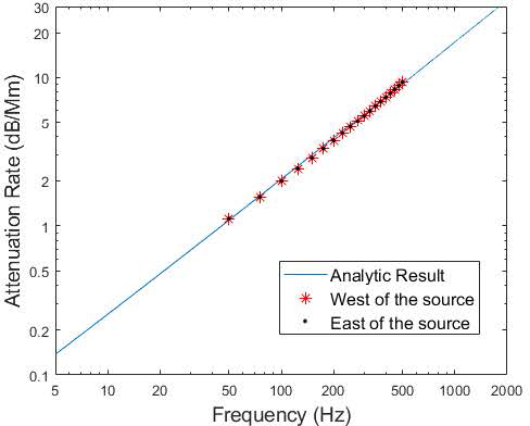
Figure 4: Comparison between the FDTD-calculated ELF propagation attenuation versus frequency over paths A $_{1 E}$ B $_{1 E}$ and A $_{1 W}$ B $_{1 W}$ with analytical results reported in [24], where the subscripts refer to the different propagation paths shown in Fig. 2.

IV. CONCLUSION

A new global FDTD model was introduced that is advantageous for long-time-span applications as well as applications that will extend over large radial distances (a wide range of altitudes). This grid arrangement is termed the global Courant-limit model because it runs at the Courant limit, the maximum permissible time step that is free from instabilities. The model was described and validated by comparing the FDTD-calculated frequency attenuation with corresponding analytical and measurement data in the literature [24].

As part of our ongoing work, we are using this model to investigate magnetotelluric and geoelectric fields at the surface of the Earth during geomagnetic storms. By coupling this model with other models, such as the Block Adaptive Tree Solar wind Roe-type Upwind Scheme (BATS-R-US) model [28–31], this model may help serve as an essential forecasting tool for predicting space weather hazards to near-Earth electrotechnologies [32].

ACKNOWLEDGMENT

This material is based upon work sponsored by the National Science Foundation under Grant 1662318. The authors would like to acknowledge high-performance computing support from Cheyenne (doi:10.5065/D6RX99HX) provided by NCAR’s Computational and Information Systems Laboratory. Also, the support and resources from the Center for High Performance Computing at the University of Utah are gratefully acknowledged.

REFERENCES

[1] K. G. Budden, The Wave-Guide Mode Theory of Wave Propagation, London: Logos Press,1961.

[2] P. B. Morris, R. R. Gupta, R. S. Warren, and P. M. Creamer, Omega Navigation System Course Book Vols. 1 and 2. Reading, MA: Analytical Sciences Corp.

[3] M. A. Tyler, “Round-the-world high frequency propagation: A synoptic study, DSTO-RR-0059,” 1995.

[4] R. W. Moses, “The high-latitude ionosphere and its effects on radio propagation,” Eos, Transactions American Geophysical Union, vol. 85, no. 19, p. 192, 2004.

[5] M. B. Cohen, U. S. Inan, R. K. Said, and T. Gjestland, “Geolocation of terrestrial gamma-ray flash source lightning,” Geophysical Research Letters, vol. 37, no. 2, 2010.

[6] L. Liebermann, “Extremely low-frequency electromagnetic waves. I. Reception from lightning,” Journal of Applied Physics, vol. 27, no. 12, pp. 1473-1476, 2004.

[7] S. A. Cummer, U. S. Inan, T. F. Bell, and C. P. Barrington-Leigh, “ELF radiation produced by electrical currents in sprites,” Geophysical Research Letters, vol. 25, no. 8, pp. 1281-1284, 1998.

[8] S. A. Cummer, U. S. Inan, and T. F. Bell, “Ionospheric D region remote sensing using VLF radio atmospherics,” Radio Science, vol. 33, no. 6, pp. 1781-1792, 1998.

[9] A. Taflove and S. C. Hagness, “Computational Electromagnetics: The Finite-Difference Time-Domain Method,” 3rd ed. Norwood, MA: Artech House, Inc., p. 1038, 2005.

[10] M. Hayakawa and T. Otsuyama, “FDTD analysis of ELF wave propagation in inhomogeneous subionospheric waveguide models,” Applied Computational Electromagnetics Society (ACES) Journal, vol. 17, no. 3, pp. 239-244, 2002.

[11] J. J. Simpson and A. Taflove, “Three-dimensional FDTD modeling of impulsive ELF propagation about the Earth-sphere,” IEEE Transactions on Antennas and Propagation, vol. 52, no. 2, pp. 443-451, 2004.

[12] J. J. Simpson, R. P. Heikes, and A. Taflove, “FDTD modeling of a novel ELF radar for major oil deposits using a three-dimensional geodesic grid of the Earth-ionosphere waveguide,” IEEE Transactions on Antennas and Propagation, vol. 54, no. 6, pp. 1734-1741, 2006.

[13] J. J. Simpson, “Current and future applications of 3-D global Earth-ionosphere models based on the full-vector Maxwell’s equations FDTD method,” Surveys in Geophysics, vol. 30, no. 2, pp. 105-130, 2009.

[14] C. Yue and Q. Zong, “Solar wind parameters and geomagnetic indices for four different interplanetary shock/ICME structures,” Journal of Geophysical Research: Space Physics, vol. 116, no. A12, 2011.

[15] J. T. Gosling, “The solar flare myth,” Journal of Geophysical Research: Space Physics, vol. 98, no. A11, pp. 18937-18949, 1993.

[16] F. Zheng, Z. Chen, and J. Zhang, “A finite-difference time-domain method without the Courant stability conditions,” IEEE Microwave and Guided Wave Letters, vol. 9, no. 11, pp. 441-443, 1999.

[17] C. C.-P. Chen, T.-W. Lee, N. Murugesan, and S. C. Hagness, “Generalized FDTD-ADI: An unconditionally stable full-wave Maxwell’s equations solver for VLSI interconnect modeling,” in IEEE/ACM International Conference on Computer Aided Design. ICCAD - 2000. IEEE/ACM Digest of Technical Papers (Cat. No.00CH37140) IEEE [Online]. Available: https://ieeexplore.ieee.org/document/896466/.

[18] Y. Yang, R. S. Chen, Z. B. Ye, and Z. B. Wang, “Analysis of planar antennas using unconditionally stable three-dimensional ADI-FDTD method,” in 2005 IEEE Antennas and Propagation Society International Symposium, 2005: IEEE [Online]. Available: https://ieeexplore.ieee.org/document/1551512/.

[19] D. L. Paul and C. J. Railton, “Spherical ADI FDTD method with application to propagation in the Earth ionosphere cavity,” IEEE Transactions on Antennas and Propagation, vol. 60, no. 1, pp. 310-317, 2012.

[20] M. A. Clilverd, C. J. Rodger, R. Gamble, N. P. Meredith, M. Parrot, J.-J. Berthelier, and N. R. Thomson, “Ground-based transmitter signals observed from space: Ducted or nonducted?,” Journal of Geophysical Research: Space Physics, vol. 113, no. A4, 2008.

[21] G. V. Khazanov, M. W. Chen, C. L. Lemon, and D. G. Sibeck, “The magnetosphere-ionosphere electron precipitation dynamics and their geospace consequences during the 17 March 2013 storm,”Journal of Geophysical Research: Space Physics, vol. 124, no. 8, pp. 6504-6523, 2019.

[22] T. Xiao and Q. H. Liu, “A Staggered Upwind Embedded Boundary (SUEB) method to eliminate the FDTD staircasing error,” IEEE Transactions on Antennas and Propagation, vol. 52, no. 3, pp. 730-741, 2004.

[23] K. H. Dridi, J. S. Hesthaven, and A. Ditkowski, “Staircase-free finite-difference time-domain formulation for general materials in complex geometries,” IEEE Transactions on Antennas and Propagation, vol. 49, no. 5, pp. 749-756, 2001.

[24] P. R. Bannister, “ELF propagation update,” IEEE Journal of Oceanic Engineering, vol. 9, 1984.

[25] J. J. Simpson and A. Taflove, “Efficient modeling of impulsive ELF antipodal propagation about the Earth sphere using an optimized two-dimensional geodesic FDTD grid,” IEEE Antennas and Wireless Propagation Letters, vol. 3, no. 1, pp. 215-218, 2004.

[26] P. R. Bannister, “The determination of representative ionospheric conductivity parameters for ELF propagation in the Earth-ionosphere waveguide,” Radio Science, vol. 20, no. 4, pp. 977-984, 1985.

[27] D. Shepard, “A two-dimensional interpolation function for irregularly-spaced data,” in Proceedings of the 1968 23rd ACM National Conference, New York: ACM Press, 1968.

[28] G. Tóth, D. L. De Zeeuw, T. I. Gombosi, W. B. Manchester, A. J. Ridley, I. V. Sokolov, and I. I. Roussev, “Sun-to-thermosphere simulation of the 28-30 October 2003 storm with the Space Weather Modeling Framework,” Space Weather, vol. 5, no. 6, 2007.

[29] K. G. Powell, P. L. Roe, T. J. Linde, T. I. Gombosi, and D. L. De Zeeuw, “A solution-adaptive upwind scheme for ideal magnetohydrodynamics,” Journal of Computational Physics, vol. 154, no. 2, pp. 284-309, 1999.

[30] T. I. Gombosi, G. Tóth, D. L. De Zeeuw, K. C. Hansen, K. Kabin, and K. G. Powell, “Semirelativistic magnetohydrodynamics and physics-based convergence acceleration,” Journal of Computational Physics, vol. 177, no. 1, pp. 176-205, 2002.

[31] T. I. Gombosi, K. G. Powell, D. L. De Zeeuw, C. R. Clauer, K. C. Hansen, W. B. Manchester, A. J. Ridley, I. I. Roussev, I. V. Sokolov, Q. F. Stout, and G. Toth, “Solution-adaptive magnetohydrodynamics for space plasmas: Sun-to-Earth simulations,” Computing in Science & Engineering, vol. 6, no. 2, pp. 14-35, 2004.

[32] M. W. Liemohn, D. T. Welling, J. J. Simpson, R. Ilie, B. J. Anderson, S. Zou, N. Y. Ganushkina, A. J. Ridley, J. W. Gjerloev, A. Kelbert, M. Burleigh, A. Mukhopadhyay, and H. Xu, “CHARGED: Understanding the Physics of Extreme Geomagnetically Induced Currents,” presented at the American Geophysical Union Fall Meeting December 01, 2018 [Online]. Available: https://ui.adsabs.harvard.edu/abs/2018AGUFMNH31C0993L

BIOGRAPHIES

Yisong Zhang received the B.S. and M.S. degrees in electrical and computer engineering from University of Utah, Salt Lake City, UT, USA, in 2017 and 2021, respectively. He is currently pursuing the Ph.D. degree in electrical and computer engineering at University of Utah.

His current research interests include finite-different time-domain modeling of geomagnetic induced current, numerical model acceleration.

Dallin R. Smith received the B.S. degree in physics from Brighton Young University at Provo, Provo, UT, USA, in 2016, and the M.S. and Ph.D. degrees in electrical and computer engineering from the University of Utah, Salt Lake City, UT, USA, in 2019 and 2020, respectively.

He is currently with the Air Force Research Laboratory, Kirkland Air Force Base, Albuquerque, NM, USA. He is currently a Research Electrical Engineer with the Ionospheric Impacts Branch, Space Vehicles Directorate. His current research involves full-wave analysis of radio wave propagation in perturbed ionosphere conditions at high and equatorial latitudes of the Earth.

Jamesina J. Simpson received the B.S. and Ph.D. degrees in electrical engineering from Northwestern University, Evanston, IL, USA, in 2003 and 2007, respectively. She is currently a Professor in the Electrical and Computer Engineering Department, University of Utah, Salt Lake City, USA. Her research lab encompasses the application of Maxwell’s equations finite-difference time-domain (FDTD) method to a wide variety of scientific and engineering applications across the electromagnetic spectrum.

Dr. Simpson received a 2010 NSF CAREER award, the 2012 IEEE AP-S Donald G. Dudley, Jr. Undergraduate Teaching Award, the 2017 International Union of Radio Science (URSI) Santimay Basu Medal, and the 2020 IEEE AP-S Lot Shafai Mid-Career Award.