A Novel 3-D DGTD-FDTD Hybrid Method withOne Overlapping Virtual Layer
Qingkai Wu, Kunyi Wang, Zhongchao Lin, Yu Zhang, and Xunwang Zhao
School of Electronic Engineering
Xidian University, Xi’an, 710071, China
wuqingkai@stu.xidian.edu.cn, zclin@xidian.edu.com
Submitted On: June 9, 2023; Accepted On: November 21, 2023
ABSTRACT
Compared with the traditional finite difference time-domain (FDTD) method, the discontinuous Galerkin time-domain (DGTD) method may face the issue of intense computation. In this paper, a novel 3-D DGTD-FDTD hybrid method is proposed to dramatically reduce the unknowns of the DGTD method. Instead of the common mass-lumped elements, this virtual layer of the Yee grid is implemented on the intersecting boundary, which simplifies the mesh generation and reduces the number of unknowns. To validate the proposed method, two examples of sphere scattering and horn antenna are considered. The simulation results demonstrate the effectiveness of the proposed method.
Index Terms: Discontinuous Galerkin time-domain method, finite-difference time-domain method, hybrid method, transient analysis.
I. INTRODUCTION
The discontinuous Galerkin time-domain (DGTD) method is a transient numerical method with high accuracy and has been reported extensively in recent years [1–3]. The DGTD method is capable of using unstructured meshes resembling the finite-element time-domain (FETD) method [4], which enables it to solve models with complex structures and maintain high accuracy at the same time. Numerical fluxes are employed in the DGTD method to separate unknowns shared among adjacent elements, allowing them to be independent. Therefore, explicit time integration schemes such as leapfrog scheme can be used in the DGTD method [5] as in the FDTD method [6, 20]. However, with an increase in the number of computing elements, the unknowns of the DGTD method will inevitably rise, and consequently the computational efficiency will decrease.
The traditional way to reduce the unknowns of DGTD method is to use the hybrid mesh instead of the unstructured mesh in single form [7]. An alternative approach is using different forms of basis functions for different types of meshes to reduce the total number of unknowns [8]. However, in most cases, the resulting computational efficiency is still limited. A more recent novel idea is to use the FDTD method to deal with hexahedral elements in hybrid mesh [9]. This idea makes use of the fast and simple characteristics of the FDTD method, and avoids the staircasing error of the FDTD method, which is more direct and effective than the traditional method of reducing unknowns. This scheme has been verified by comparing the results with those obtained by FETD [9–13]. The standard procedure requires the grids in the common area should be divided into tetrahedral elements for the FETD method. A similar operation was introduced into the solution of the DGTD method [14] in recent years. It achieves good results by one common buffer. However, the existence of instance buffer [14–16] hinders the generation of hybrid meshes and efficiency.
In this paper, a novel three-dimension explicit DGTD-FDTD hybrid method is proposed. There is only one overlapping virtual layer of the FDTD zone between the DGTD and the FDTD zone to replace the buffer zone. Thereby the calculation of electromagnetic fields towards FDTD zone shares similarities with the domain decomposition FDTD (DD-FDTD) method detailed in [17, 18]. The electromagnetic fields from the FDTD zone are converted to numerical fluxes and added into DGTD’s formulations. Moreover, the tetrahedral elements used in the DGTD zone can be generated more freely, and it is not required to generate additional elements [13] to meet the mass-lumped element’s standard. Such a procedure saves considerable computation time compared with traditional hybrid strategy. To validate the proposed strategy, two examples are presented in this paper. The comparison of different methods’ results validates this method’s accuracy and high performance.
II. THE FORMULATION OF DGTD
After testing by the discontinuous Galerkin method, the weighted integral form of source free Maxwell equations are
| (1) |
Here, v is the weight function, represents the permittivity, is permeability, and denotes the space of the tetrahedral element.
The numerical fluxes with respect to element I is defined at the element boundary. j represents the adjacent element of element i.
| (2) | |||||
Here, is the unit outward normal vector of face of the element i. E and H represent the numerical fluxes, Z is the impedance and Y is the admittance.
The integral procedure results in
| (3) |
By substituting equation (3) into equation (1) we obtain the Maxwell-DGTD equation in matrix form
| (4) |
Here, E and H are expanded by the 2nd-order hierarchical basis function, defined in [19], M denotes the mass matrix, S denotes the stiffness matrix, F, F, F and F are the numerical flux matrices, represents the permittivity, is permeability, j represents the adjacent element of element i, and p is the number of the surface of the tetrahedral elements.
The leapfrog scheme has been adopted in the iteration process. Furthermore, Equation (1) can be converted into the explicit scheme as follows:
| (5) |
represents the inverse of the mass matrix. and denote the reciprocals of permittivity and permeability.
III. VIRTUAL LAYER STRATEGY FOR DGTD-FDTD HYBRID METHOD
A. DGTD-FDTD hybrid strategy
As shown in Fig. 1 (a), a hybrid strategy is proposed. One layer of FDTD Yee grids will be set as the virtual layer, and the virtual layer overlaps the tetrahedral DGTD elements. Since the generation of tetrahedral mesh in the DGTD zone will not be affected by the virtual layer, the tetrahedron elements can be directly connected. While the conventional needs one extra hybrid region, the grid needs to be split into six tetrahedral elements. As a result, the split elements will add obvious unknowns.
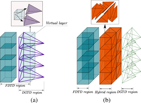
Figure 1: Two types of hybrid mesh: (a) The virtual layer hybrid mesh and (b) the conventional hybrid mesh.
In the conventional hybrid method, the hybrid region is calculated by a new algorithm merged from DGTD and FDTD method. A new mass matrix is built by both basis functions in DGTD and the field-components in FDTD.
| (6) |
In Equation (6), M and Mrepresent the respective mass matrix. And the Mis calculated by the projection of the overlapped basis functions and field-components. The FDTD method is simple and fast. So we convert the 3-D hybrid problem into two 2-D problems and keep the characteristics of FDTD at the same time.
In our proposed method, we apply a concise strategy to communicate DGTD and FDTD zones. The fields from the FDTD zone will be transmitted through the boundary of two types of meshes to the DGTD zone. The fields from the DGTD zone will be transmitted on the red face of the virtual layer to the FDTD zone. Consequently, there will be no mutual interference during the communication of the two methods based on the virtual layer hybrid strategy.
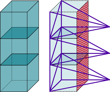
Figure 2: The locations of the electric field denoted by red arrows in virtual layer.
In Fig. 2, when the FDTD zone needs to update the fields, it will use the electric field (E-field) from the face (indicated with red). The E-field for FDTD method on the face of the virtual layer, meanwhile inside the overlapping DGTD zone, can be directly calculated by the DGTD method in explicit scheme, using . E represents the vector field in the DGTD zone, N stands for the basis functions, and e is the expansion coefficients [19].
The electromagnetic fields from the FDTD zone to the DGTD zone must be converted to the form of numerical fluxes. Specifically, the fields from the FDTD zone will be approximated by fields value averaged spatially. The edge basis function will directly use the field value of FDTD zone due to the application of hierarchical basis functions. Correspondingly, the field value of the hypotenuse edge inside the square is the average value of the surrounding electric fields (E-field) following [8]. Besides, the magnetic field (H-field) should be averaged from the real and virtual zone of FDTD in order to maintain time consistency to avoid the error accumulation from the inconsistency in time. The entire calculation process is exhibited in Fig. 3.
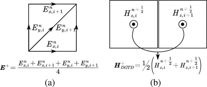
Figure 3: The assembly of FDTD EH-fields for DGTD zone: (a) The constituent components of E and (b) the constituent components of H.
The E or H (see Fig. 3) will be treated as the E or H to introduce into the numerical fluxes in Eq. (2) to update fields.
B. Generation of hybrid mesh
To generate the hybrid mesh with one virtual layer, we follow the procedure in Fig. 4. Firstly, in the whole computation domain, the structured grids used for the FDTD method will be divided, and then the grids intersecting with the object should be dug out based on the geometric contour of the object (surrounded by the blue line). After that, the innermost layer of structured grids is set as the virtual layer (between blue and red lines). Finally, the region inside the red lines is set as the DGTD region, and tetrahedral elements will be generated there.
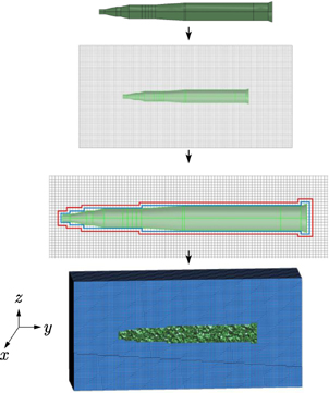
Figure 4: The mesh of DGTD-FDTD hybrid zone. The operation of dividing grids. The comparison of hybrid mesh in 2-D.
C. The marching-on-in-time algorithm
To ensure that the combination of the two methods is self-consistent, the following process of explicit iteration has been implemented:
FDTD and DGTD method will iterate normally when they are not in the overlapping zone.
In the overlapping zone, updating of the E-field for two methods is as follows:
1) DGTD should update the E-field on the inner face of the virtual layer.
2) FDTD method updates the E-fields.
3) Fields from the FDTD zone should be combined and converted to the form of numerical fluxes for the updated H-field in the DGTD zone.
Updating of the H-field for two methods:
1) DGTD should update the H-field on the inner face of the virtual layer.
2) FDTD method updates the H-fields.
3) Fields from the FDTD zone should be combined and converted to the form of numerical fluxes for the next iteration’s updated E-field in the DGTD zone.
Since the explicit iteration scheme is employed here, the t in the presented work is chosen based on the following rule:
| (7) |
The choice of tfollows the rule in [6], The selection of t satisfies the Lemma 2.9 in [21]:
| (8) |
In Eq. (8), and are coefficients obtained by [21], V and P are the volume and the total area of the element i, respectively, is the permittivity of the element i, is the permeability of the element i, the superscript ”+” indicates the adjacent elements of the element i.
Because the calculation of hybrid region doesn’t involve new algorithms, the selection of t just needs to satisfy the CFL (Courant-Friedrichs-Lewy) conditions [6].
IV. NUMERICAL RESULTS
All of the numerical simulations were carried out on the Intel Xeon Gold 6140 CPU @ 2.30 GHz with 64 GB of RAM. And the programming language is implemented in Fortran 95.
A. Sphere scattering
In this example, a perfect electric conductor (PEC) sphere’s bistatic scattering is computed by different methods. This sphere’s radius is 0.5 m, and the planewave’s propagation direction is -z. Figure 5 represents the grids and tetrahedrons of the sphere model. The outermost five layers of the FDTD zone are set as the uniaxial perfectly matched layer (UPML) boundary. Correspondingly, the comparison model of the DGTD method is truncated by five UMPL layers, too, as illustrated in Fig. 5. The mesh size of both models’ tetrahedral elements is /10; the Yee grids in all models are generated with mesh size /15. In addition, the FDTD method used a conformal algorithm [22] to improve accuracy.
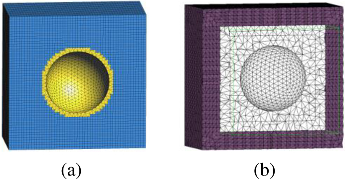
Figure 5: Mesh of different methods: (a) The mesh of hybrid method and (b) the mesh of conventional DGTD method.
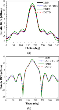
Figure 6: Comparison of bistatic RCS computed by different methods: (a) xoz plane and (b) yoz plane.
The comparison of bistatic scattering of different methods at the frequency of 400 MHz is highlighted in Fig. 6. Based on the results of this comparison, it can be inferred that the results of the hybrid method and method of moment (MoM) are in good agreement, and it has prominently better results than the FDTD method. It can be found that the hybrid method has an obvious improvement on accuracy when compared with the FDTD method. Results of the comparison between the conventional DGTD method and the proposed method are listed in Table 1. It is evident that the proposed method has a tremendous advantage compared with the conventional DGTD method. The proposed method is 20 times faster than the DGTD method, which significantly reduces the computation memory and improves the efficiency. On the other hand, due to the virtual layer, the proposed method can save calculation time significantly compared with the conventional strategy.
Table 1: Performance of Different Methods
| Method | Memory (MB) | Unknowns | Solution Time (s) |
|---|---|---|---|
| DGTD | 9283 | 11,435,600 | 10,901 |
| Conventional method (with buffer zone) | 1504 | 1,190,454 | 757 |
| Proposed method | 1037 | 861,134 | 522 |
B. Horn antenna
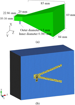
Figure 7: The horn antenna model: (a) The model with the geometric size of the horn antenna and (b) the hybrid mesh for DGTD-FDTD method.
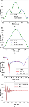
Figure 8: The comparison of different methods: (a) The gain pattern of xoz-plane, (b) the gain pattern of yoz-plane, (c) the result of S-parameter and (d) the time-domain result of port’s voltage.
The second example is a horn antenna. It is one kind of broadband antenna. Because of its opening structure, it is quite suitable for computation with the proposed hybrid method. Figure 7 represents the hybrid mesh of the horn antenna model. The mesh size of both models’ tetrahedral elements is ; the mesh size of the Yee grids for FDTD method in both models is .
A coaxial wave port is used to excite the antenna, which is inside the DGTD zone. The exciting signal is chosen as a modulated Gaussian pulse with bandwidth of 515 GHz. From Figs. 8 (a)-(c), we can find that the gain pattern and S-parameter of the proposed DGTD-FDTD hybrid method is in good agreement with the finite element method (FEM) and DGTD method. In Fig. 8 (d), the comparison of port’s voltage of DGTD and DGTD-FDTD method is given to prove the stability of hybrid method. From Table 2, the results demonstrate that the hybrid method still has a significant advantage in the unknowns compared with the DGTD method. From the comparison, the proposed method exhibits a 15.28 times improvement in overall computing efficiency and nearly 13 times improvement in memory usage.
Table 2: Performance of different methods
| Method | Memory (MB) | Unknowns | Solution Time (s) |
|---|---|---|---|
| FEM | 5431 | 1,359,660 | 1523 |
| DGTD | 26,150 | 8,377,240 | 14,732 |
| The conventional method | 2340 | 751,330 | 1315 |
| The proposed method | 2132 | 626,944 | 964 |
V. CONCLUSION
In this paper, a novel 3-D hybrid method of the DGTD and FDTD method is introduced. One virtual layer of FDTD has been adapted to maintain the independence of the communication between the two methods. On this premise, it is not necessary to add additional elements for the actual common buffer as it is the conventional hybrid method. Consequently the unknowns will obviously be reduced. As a result, there will be a significant improvement in memory usage and computational efficiency compared with the conventional DGTD method and hybrid method.
ACKNOWLEDGMENT
This work was supported in part by Key Research and Development Program of Shaanxi (2022ZDLGY02-01, 2021GXLH-02, 2023-ZDLGY-09,) and the Fundamental Research Funds for the Central Universities (QTZX23018).
REFERENCES
[1] J. S. Hesthaven and T. Warburton, Nodal Discontinuous Galerkin Methods: Algorithms, Analysis, and Applications. New York, NY, USA: Springer, pp. 1-39, 2008.
[2] S. Dosopoulos and J.-F. Lee, “Interior penalty discontinuous Galerkin finite element method for the time-dependent first-order Maxwell’s equations,” IEEE Trans. Antennas Propag., vol. 58, no. 12, pp. 4085-4090, Dec. 2010.
[3] M. Li, Q. Wu, Z. Lin, Y. Zhang, and X. Zhao, “A minimal round-trip strategy based on graph matching for parallel DGTD method with local time-stepping,” IEEE Antennas Wirel Propag Lett., vol. 2, pp. 243-247, Feb. 2023.
[4] J.-M. Jin, The Finite Element Method in Electromagnetics. Hoboken, NJ, USA: Wiley, pp. 514-523, 2015.
[5] J. Chen and Q. Liu, “Discontinuous Galerkin time-domain methods for multiscale electromagnetic simulations: A review,” Proc. IEEE, vol. 101, no. 2, pp. 242-254, Feb. 2013.
[6] A. Taflove and S. C. Hagness, Computational Electrodynamics: The Finite-difference Time-Domain Method. Norwood, MA, USA: Artech House, pp. 638-649, 2005.
[7] F. Hassan, “High-order discontinuous Galerkin method for time-domain electromagnetics on non-conforming hybrid meshes,” Math Comput Simul., no. 107, pp. 134-156, Jan. 2015.
[8] Z. Xiao, B. Wei, and D. Ge, “A hybrid mesh DGTD algorithm based on virtual element for tetrahedron and hexahedron,” IEEE Trans. Antennas Propag., vol. 69, no. 4, pp. 2242-2248, Apr. 2021.
[9] D. S. Balsara and J. J. Simpson, “Making a synthesis of FDTD and DGTD schemes for computational electromagnetics,” in IEEE J Multiscale Multiphys Comput Tech., vol. 5, pp. 99-118, June2020.
[10] T. Rylander and A. Bondeson, “Stable FEM-FDTD hybrid method for Maxwell’s equations,” in Comput. Phys. Commun., vol. 125, no. 1-3, pp. 75-82, Mar. 2000.
[11] J. Wang, Q. Ren, and F. Dai, “3-D hybrid finite-difference time-domain (FDTD)/wave equation finite element time-domain (WE-FETD) method,” Int. Symp. on Antennas, Propag and EM Theory (ISAPE), pp. 1-2, 2021.
[12] N. V. Venkatarayalu, G. Y. Beng, and L.-W. Li, “On the numerical errors in the 2-D FE/FDTD algorithm for different hybridization schemes,” IEEE Microw. Wireless Compon. Lett., vol. 14, no. 4, pp. 168–170, Apr. 2004.
[13] A. Sharbaf and R. Sarraf-Shirazi, “An unconditionally stable hybrid FETD-FDTD formulation based on the alternating-direction implicit algorithm,” IEEE Antennas Wirel Propag Lett., vol. 9, pp. 1174-1177, Dec. 2010.
[14] S. G. Garcia, M. F. Pantoja, C. M. de Jong van Coevorden, A. R. Bretones, and R. G. Martin, “A new hybrid DGTD/FDTD method in 2-D,” in IEEE Microw. Wireless Compon. Lett., vol. 18, no. 12, pp. 764-766, Dec. 2008.
[15] Q. Sun, Q. Ren, Q. Zhan, and Q. H. Liu, “3-D domain decomposition based hybrid finite-difference time-domain/finite-element time-domain method with nonconformal meshes,” IEEE Trans. Microw. Theory Techn., vol. 65, no. 10, pp. 3682-3688, Apr. 2017.
[16] B. Zhu, J. Chen, W. Zhong, and Q. Liu, “A hybrid FETD-FDTD method with nonconforming meshes,” Commun Comput Phys., vol. 9, no. 3, pp. 828-842, Mar. 2011.
[17] K. S. Yee, J. S Chen, and A. H. Chang, “Conformal finite-different time-domain (FDTD) with overlapping grids,” IEEE Trans. Antennas Propag., vol. 40, no. 9, pp. 1068-1075, Sep. 1992.
[18] F. Xu and W. Hong, “Domain decomposition FDTD algorithm for the analysis of a new type of E-plane sectorial horn with aperture field distribution optimization,” IEEE Trans. Antennas Propag., vol. 52, no. 2, pp. 426-434, Feb. 2004.
[19] Y. Zhou, R. Huang, S. Wang, Q. Ren, W. Zhang, G. Yang, and Q. H. Liu, “An adaptive DGTD algorithm based on hierarchical vector basis function,” in IEEE Trans. Antennas Propag., vol. 69, no. 12, pp. 9038-9042, Dec. 2021.
[20] J. Alvarez, L. D. Angulo, M. F. Pantoja, A. R. Bretones, and S. G. Garcia, “Source and boundary implementation in vector and scalar DGTD,” in IEEE Trans. Antennas Propag, vol. 58, no. 6, pp. 1997-2003, June 2010.
[21] L. Fezoui, S. Lanteri, S. Lohrengel, and S. Piperno, “Convergence and stability of a discontinuous Galerkin time-domain method for the 3D heterogeneous Maxwell equations on unstructured meshes,” ESAIM, Math. Model Numer. Anal., vol. 39, no. 6, pp. 1149-1176, Nov. 2005.
[22] S. Dey and R. Mittra, “A modified locally conformal finite-difference time-domain algorithm for modeling three-dimensional perfectly conducting objects,” in IEEE Microwave Opt. Tech. Lett, vol. 7, no. 9, pp. 273-275, June 1997.
BIOGRAPHIES

Qingkai Wu was born in Yangzhou, Jiangsu, China, in 1997. He received the B.S. degree in electronic science and technology from Xidian University, Xi’an, China, in 2020. He is currently pursuing the Ph.D. degree with Xidian University, Xi’an, China. His current research interests include transient electromagnetic analysis.

Kunyi Wang was born in Anqing, Anhui, China, in 1996. He received the B.S. degree in electronic information engineering from Tianjin University of Technology, Tianjin, China, in 2019. He is currently pursuing the Ph.D. degree with Xidian University, Xi’an, China. His current research interests include transient electromagnetic analysis.

Zhongchao Lin was born in Hubei, China, in 1988. He received the B.S. and Ph.D. degrees from Xidian University, Xi’an, China, in 2011 and 2016, respectively. He joined Xidian University, in 2016, as a post doctoral fellow, where he was lately promoted as an associate professor. His research interests include large-scale computational electromagnetics, scattering, and radiation electromagnetic analysis.

Yu Zhang received the B.S., M.S., and Ph.D. degrees from Xidian University, Xi’an, China, in 1999, 2002, and 2004, respectively. In 2004, he joined Xidian University as a faculty member. He was a visiting scholar and an adjunct professor with Syracuse University from 2006 to 2009. As a principal investigator, he works on projects, including the Project of NSFC. He has authored four books: Parallel Computation in Electromagnetics (Xidian University Press, 2006), Parallel Solution of Integral Equation-Based EM Problems in the Frequency Domain (Wiley IEEE, 2009), Time and Frequency Domain Solutions of EM Problems Using Integral Equations and a Hybrid Methodology (Wiley, 2010), and Higher Order Basis Based Integral Equation Solver (Wiley, 2012), as well as more than 100 journal articles and 40 conference papers.

Xunwang Zhao was born in Shanxi, China, in 1983. He received the B.S. and Ph.D. degrees from Xidian University, Xi’an, China, in 2004 and 2008, respectively. He joined Xidian University, in 2008, as a faculty member, where he was lately promoted as a full professor. He was a visiting scholar with Syracuse University, Syracuse, NY, USA, from December 2008 to April 2009. As a principal inves tigator, he works on several projects, including the project of NSFC. His research interests include computational electromagnetics and electromagnetic scattering analysis.
ACES JOURNAL, Vol. 38, No. 8, 558–565
doi: 10.13052/2023.ACES.J.380802
© 2023 River Publishers