A Note on Matrix Decomposition for Synthetic Basis Functions Method in the Analysis of Periodic Structures

Yanlin Xu${}^{\mathbf{\text{1}}}$, Ning Hu${}^{\mathbf{\text{2}}}$, Chenxi Liu${}^{\mathbf{\text{1}}}$, Hao Ding${}^{\mathbf{\text{1}}}$, and Jun Li${}^{\mathbf{\text{3}}}$

¹College of Electronic Science and Technology
National University of Defense Technology, Changsha 410073, China
13298656824@163.com, liuchenxi09@nudt.edu.cn, dinghao20a@nudt.edu.cn

²Information Engineering University
Zhengzhou 450001, China
1141832906@qq.com

³The Second Representative Office of Changsha Area
Changsha 410011, China
271069796@qq.com

Submitted On: June 9, 2023; Accepted On: September 16, 2024

ABSTRACT

The synthetic basis functions method (SBFM) is discussed in this work and orthogonal triangle decomposition (QR decomposition) is adopted to extract independent items from solution space in the construction of synthetic functions. Just like singular value decomposition (SVD), accuracy of SBFM+QR improves with the growth of the number of synthetic functions. However, there is an interesting phenomenon for SBFM+QR: only one synthetic function is enough to get the same level of accuracy with method of moments (MoM) when a single body is concerned. Moreover, this feature can be further extended to periodic arrays. In other words, for periodic arrays, one synthetic function is enough to get high accuracy if SBFM+QR is adopted. This is meaningful for large-scale periodic arrays and may lead to benefits such as decreasing memory cost and improving efficiency.

Index Terms: Matrix decomposition, method of moments, periodic structures, surface integral equation, synthetic functions.

I. INTRODUCTION

Fast and accurate analysis of large-scale periodic arrays is an appealing and challenging task in computational electromagnetics. Method of moments (MoM) is a classical numerical approach well known for high accuracy. However, traditional MoM is hardly applied in the analysis of large-scale problems due to the restrictions on computational complexity and memory cost. To make MoM suitable for large-scale problems, many approaches have been proposed in the past decades [1–10]. The synthetic basis functions method (SBFM) is of special interest [11–20].

In contrast to traditional MoM, synthetic functions (SFs) are adopted in SBFM to discretize unknown vectors and to make the Galerkin test yield a high compressed matrix equation. Thus, the memory cost of SBFM will be decreased sharply. This makes it possible to analyze large-scale problems on a single PC. Similar approaches such as the sub-entire-domain (SED) basis functions method [21] and the characteristic basis functions method (CBFM) [22, 23] can be found in related literature and we are not going to introduce them in detail for the sake of brevity.

SBFM was initially presented by Matekovits et al. in 2001 in the analysis of array antennas [11]. A systematic work on SBFM was published in 2007 by Matekovits et al. which perfected the theory of SBFM [12]. Thereafter, SBFM concerned many scholars and a series of improved works were presented [13–20]. In SBFM, the construction of SFs is a core problem. Initially, Matekovits et al. defined SFs as linear combinations of a series of low order basis functions. Then, the solution space of SFs can be obtained by solving the responses of targets to excitations. Finally, singular value decomposition (SVD) can be implemented to extract independent items from the solution space which yields the expansion coefficient matrix of SFs.

In this paper, emphasis is on the matrix decomposition and orthogonal triangle decomposition (QR decomposition) is used to extract independent items from the solution space. From the results we find that, in general, accuracy of SBFM+QR improves with the growth of the number of SFs and this is coincident with the case of SBFM+SVD. We also found an interesting phenomenon: if the target is a single body with one natural excitation, one SF is enough for SBFM+QR to get the same level of accuracy with traditional MoM. Then, based on concrete theoretical analysis, we give an explanation of the phenomenon. This feature can be extended from a single body to periodic arrays at the expense of slightly lowering accuracy. Notably, compared to SBFM+SVD, if there is one natural excitation, SBFM+QR can get a high level of accuracy with only one SF. Finally, a 10$\times$10 circular microstrip patch antenna array is analyzed to validate effectiveness of the conclusion.

II. THEORY AND PHENOMENON

As SBFM is an improved approach of MoM, we will begin with the theory of MoM. Usually, the electric field integral equation (EFIE) can be written as:

$$\widehat{n}\times L(J)=\widehat{n}\times E_{\mathrm{inc}},$$

(1)

where L is the integral operator and defined as:

$$L(X)=\mathrm{j}\omega \mu {\int }_S[X+\frac{1}{k^2}\nabla (\nabla \cdot X)]gdS.$$

(2)

To solve EFIE using MoM, a series of basic functions (e.g. RWG functions) are used to discretize the unknown vector J and to make the Galerkin test. Then, equation (1) can be transformed into a linear scalar matrix equation:

$$ZI=V,$$

(3)

where Z is impedance matrix, V is exciting matrix, and I is the current coefficients of RWG functions.

Unlike MoM, SFs are used, in SBFM, to discretize the unknown vector J and to make the Galerkin test. Then, equation (1) can be transformed into a compressed matrix equation [24]:

$$\{\begin{array}{c}{W}_{\mathrm{SBF}}Y=G_{\mathrm{SBF}}\hfill \\ W_{\mathrm{SBF}}=P^{\mathrm{H}}ZP\hfill \\ G_{\mathrm{SBF}}=P^{\mathrm{H}}V\hfill \end{array},$$

(4)

where P and Y are expansion coefficients matrix and current coefficients matrix of SFs, respectively, and Z and V are impedance matrix and exciting matrix of MoM.

Equation (4) indicates that the impedance matrix W${}_{S\mathit{}B\mathit{}F}$ and exciting matrix G${}_{S\mathit{}B\mathit{}F}$ of SBFM can be found on the basis of Z and V as long as the expansion coefficients matrix P of SFs is obtained. In other words, the core of SBFM is the calculation of SFs’ expansion coefficients matrix. Here, we take a single body for demonstration.

For a specific body, assume the number of SFs and RWG functions defined on it are M and N, respectively. Usually, M $<$$<$ N. Then, SFs can be written as the linear combinations of RWG functions:

$$\left[\begin{array}{c}\hfill F_1\hfill \\ \hfill F_2\hfill \\ \hfill \mathrm{\cdots }\hfill \\ \hfill F_M\hfill \end{array}\right]=\left[\begin{array}{cccc}\hfill p_{11}\hfill & \hfill p_{12}\hfill & \hfill \mathrm{\cdots }\hfill & \hfill p_{1N}\hfill \\ \hfill p_{21}\hfill & \hfill p_{22}\hfill & \hfill \mathrm{\cdots }\hfill & \hfill p_{2N}\hfill \\ \hfill \mathrm{\cdots }\hfill & & \hfill \mathrm{\cdots }\hfill & \hfill \mathrm{\cdots }\hfill \\ \hfill p_{m1}\hfill & \hfill p_{m2}\hfill & \hfill \mathrm{\cdots }\hfill & \hfill p_{mN}\hfill \end{array}\right]\left[\begin{array}{c}\hfill f_1\hfill \\ \hfill f_2\hfill \\ \hfill \mathrm{\cdots }\hfill \\ \hfill f_N\hfill \end{array}\right].$$

(5)

Equation (5) can be compactly written as:

$${\left\{F_k\right\}}_{M\times 1}=P_{N\times M}^{\mathrm{H}}{\left\{f_k\right\}}_{N\times 1},$$

(6)

where fand F stand for the RWG functions and SFs defined on the body, and P is the expansion coefficients matrix of SFs.

To get the expansion coefficients matrix P, there are three steps.

1. Step 1: setting auxiliary exciting sources (AES).

   Initially, Matekovits et al. defined AES on a series of discrete small RWG functions around the target, as shown in Fig. 1 (a). Then, in 2010, Bo Zhang et al. defined AES on an irregularly meshed surface which makes AES with diverse polarizations, as shown in Fig. 1 (b) [14]. This is beneficial to improve accuracy, and AES will be set in the second way in this work.

   

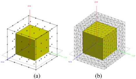
   Figure 1: A cube surrounded by a series of AES: (a) AES defined on a series of discrete small RWG functions and (b) AES defined on a meshed surface.

2. Step 2: solving solution space.

   Defining the mutual coupling impedance matrix between target and AES as V${}^e$, the solution space R of SFs can be computed as:

   $$R_{N\times (S+1)}=Z^{-1}(V+V^e),$$

   (7)

   where N is the number of RWG functions defined on the target and S represents the number of AES.

   Equation (7) shows that the solution space R contains two parts:

   1. Response to natural excitations (incident wave):

      $$r^1=Z^{-1}V.$$

      (8)

   2. Response to AES:

      $$[r^2,r^3,\mathrm{\dots },r^{S+1}]=Z^{-1}{V}^e,$$

      (9)

      where r${}^{\mathrm{i}}$ (i=1, 2,…, S+1) is the i-th column of R.

3. Step 3: extracting independent items. To extract independent items from the solution space R, SVD is usually adopted, as shown in equation (10), where $\rho {}_i$ is the i-th singular value of R and $\rho {}_1\ge \rho {}_2\ge \mathrm{\cdots }\ge \rho {}_N$:

   $$R=U\rho V^{\mathrm{H}};\rho =\mathrm{diag}({\rho }_1,{\rho }_2,\mathrm{\cdots },{\rho }_N).$$

   (10)

   Considering U is a unitary matrix, if $\rho$${}_M$/$\rho$${}_1$$<$$\rho$${}_{SBF}$, we will take the first M columns of U as the expansion coefficients matrix P of SFs, as shown in equation (11), where I${}_{\mathrm{M}}$ represents an identity matrix:

   $$P_{N\times M}=U_{N\times N}{\left[\begin{array}{c}\hfill I_M\hfill \\ \hfill 0\hfill \end{array}\right]}_{N\times M}.$$

   (11)

The truncation error $\rho$${}_{SBF}$ is usually determined by operator and, in different applications, $\rho$${}_{SBF}$ is also different.

According to equation (4), we can get the current coefficients of SFs:

$$Y=W_{\mathrm{SBF}}^{-1}{G}_{\mathrm{SBF}}={(P^{\mathrm{H}}ZP)}^{-1}{P}^{\mathrm{H}}V.$$

(12)

Then, based on equation (6), the current coefficient of RWG functions defined on the targets will be:

$$I=PY=P{(P^{\mathrm{H}}ZP)}^{-1}{P}^{\mathrm{H}}V.$$

(13)

Substituting equation (11) into equation (13) we get:

$$I=U\left[\begin{array}{c}\hfill I_M\hfill \\ \hfill 0\hfill \end{array}\right]{\left\{\left[I_M\mathrm{\hspace{0.33em}0}\right]U^{\mathrm{H}}ZU\left[\begin{array}{c}\hfill I_M\hfill \\ \hfill 0\hfill \end{array}\right]\right\}}^{-1}\left[I_M\mathrm{\hspace{0.33em}0}\right]U^{\mathrm{H}}V.$$

(14)

Equation (14) is rather interesting to us. Left multiply [I${}_{\mathrm{M}}$ 0] represents the first M rows of a matrix, and right multiply [I${}_{\mathrm{M}}$ 0]${}^H$ represents the first M columns of a matrix. Assign U${}^{\mathrm{H}}$ZU=T, the inner part of equation (14) can be rewritten as:

$${\left\{\left[I_M\mathrm{\hspace{0.33em}0}\right]U^{\mathrm{H}}ZU\left[\begin{array}{c}\hfill I_M\hfill \\ \hfill 0\hfill \end{array}\right]\right\}}^{-1}={\left\{\left[I_M\mathrm{\hspace{0.33em}0}\right]T\left[\begin{array}{c}\hfill I_M\hfill \\ \hfill 0\hfill \end{array}\right]\right\}}^{-1}=T_M{}^{-1},$$

(15)

where T${}_M$ is a sub-matrix composed of the first M rows and the first M column of T.

Substituting equation (15) into equation (14), we get:

$$I=U\left[\begin{array}{c}\hfill I_M\hfill \\ \hfill 0\hfill \end{array}\right]T_M{}^{-1}\left[I_M\mathrm{\hspace{0.33em}0}\right]U^{\mathrm{H}}V=P{T}_M{}^{-1}P^{\mathrm{H}}V.$$

(16)

From the theory of SBFM we know that, with the growth of M, current coefficients of RWG functions calculated in equation (16) will get closer and closer to that calculated by MoM.

Let us take the example in Fig. 1 (b) into consideration. There are a total of 1944 RWG functions defined on the surface of cube. Current coefficients of these RWG functions are calculated by MoM and SBFM, and the results are denoted as I${}_{MoM}$ and I${}_{SBF}$, respectively.

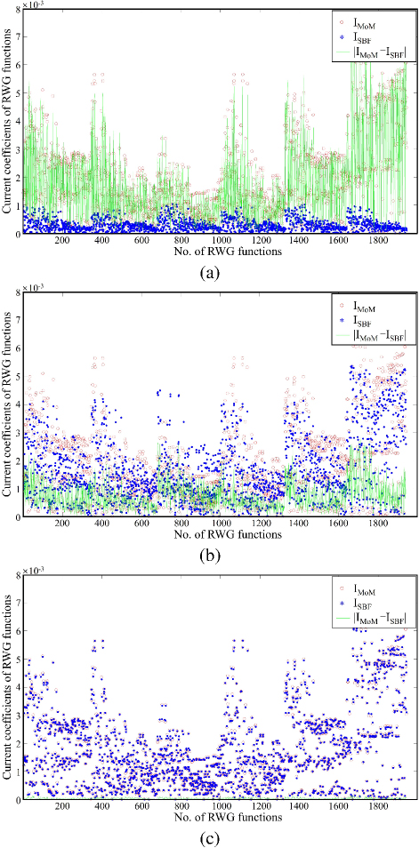
Figure 2: Absolute current coefficients of RWG functions defined on a cube in the case of SVD: (a) M=1, (b) M=50 and (c) M=150.

Figure 2 exhibits the discrepancy of I${}_{MoM}$ and I${}_{SBF}$ when different numbers of SFs are adopted. It is obvious that, with the growth of M, current coefficients of RWG functions calculated by MoM and SBFM get closer and closer which is coincident with our cognition. However, if we use QR decomposition rather than SVD to extract independent items from solution space R, as shown in equation (17), will the conclusion still be right?

$$R_{N\times (S+1)}=Q_{N\times N}{\left[\begin{array}{ccc}\hfill r_{11}\hfill & & \hfill *\hfill \\ & \hfill \mathrm{\cdots }\hfill & \\ \hfill 0\hfill & & \hfill *\hfill \end{array}\right]}_{N\times (S+1)}.$$

(17)

Similar to U, Q is also a unitary matrix and we will take the first M columns as the expansion coefficients matrix P of SFs:

$$P_{N\times M}=Q_{N\times N}{\left[\begin{array}{c}\hfill I_M\hfill \\ \hfill 0\hfill \end{array}\right]}_{N\times M}.$$

(18)

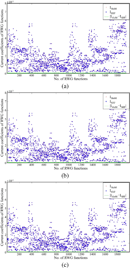
Figure 3: Absolute current coefficients of RWG functions defined on a cube in the case of QR: (a) M=1, (b) M=50, and (c) M=150.

In the case of QR decomposition, current coefficients of RWG functions defined on the surface of the cube are computed and the results are shown in Fig. 3. It is not difficult to see that accuracy of SBFM does not improve with the growth of M and current coefficients calculated by SBFM coincide exactly with those of MoM. Moreover, for SBFM, only one SF (M=1) is enough to get the same level of accuracy with MoM. This is somewhat interesting.

To further verify the above conclusion, two single models, sphere and cylinder, shown in Fig. 4, are analyzed using SBFM+SVD/QR. Similar to the cases in Figs. 2 and 3, MoM and SBFM are used to calculate the current coefficients of RWG functions defined on the surface of a sphere (1161 RWG functions) and a cylinder (1713 RWG functions). Figure 5 exhibits the absolute discrepancy of current coefficients calculated by different approaches. The results of sphere and cylinder are similar to that of cube. This suggests that the conclusions drawn from Fig. 3 may be universal. In summary, for a single body, if SBFM+QR decomposition is adopted, only one SF is enough to get the same level of accuracy with MoM.

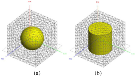
Figure 4: A target surrounded by a series of AES: (a) sphere and (b) cylinder.

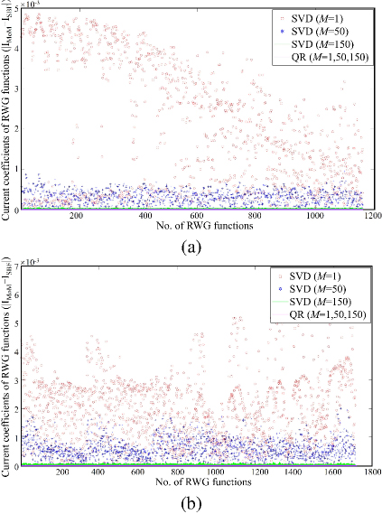
Figure 5: Absolute discrepancy of current coefficients calculated by MoM and SBFM: (a) sphere and (b) cylinder.

III. EXPLANATION AND EXPANSION

In section II, we can see that, for a single body, if QR decomposition is adopted to extract independent items from solution space, one SF is enough to get satisfying accuracy. In this section, we give a theoretical explanation on this phenomenon.

Denote Q=[q${}^{\mathrm{1}}$ q${}^{\mathrm{2}}$ … q${}^{\mathrm{N}}$], where q${}^{\mathrm{i}}$ (i=1, 2,…, N) is the i-th column of Q. According to the principle of QR decomposition, a unitary matrix and an upper triangular matrix will be yielded after decomposition, as shown in equation (17). Then, we get:

$$q^1{r}_{11}=r^1.$$

(19)

Substituting equation (8) into equation (19) to get:

$$q^1=\frac{1}{r_{11}}{Z}^{-1}V.$$

(20)

If only one SF is adopted, it will be P$\mathrm{=}$q${}^{\mathrm{1}}$. Then, according to equation (16), the current coefficients of RWG functions can be computed as:

$$I=q^1\frac{1}{t_{11}}{[q^1]}^{\mathrm{H}}V,$$

(21)

where t${}_{\mathrm{11}}$ is the element located in the first row and the first column of matrix T and T=Q${}^{\mathrm{H}}$ZQ. According to the definition of matrix T, t${}_{\mathrm{11}}$ is computed as:

$$t_{11}=\sum _{j=1}^N\sum _{i=1}^N{q}_{i1}{z}_{ij}{q}_{j1},$$

(22)

where q${}_i$${}_{\mathrm{1}}$ (i=1, 2,…, N) is the i-th element of q${}^{\mathrm{1}}$.

Then, substituting equation (20) into equation (21) and considering the results of [q${}^{\mathrm{1}}$]${}^H$V is a scalar, equation (21) can be written as:

$$I=\frac{k_e}{t_{11}}{q}^1=\frac{k_e}{t_{11}{r}_{11}}{Z}^{-1}V,$$

(23)

where k${}_e$ is a scalar and defined as k${}_e$=[q${}^{\mathrm{1}}$]${}^H$V.

For the three models shown in Figs. 1 (b) and 4, we can compute the scalar coefficients k${}_e$/(t${}_{\mathrm{11}}$r${}_{\mathrm{11}}$), as given in Table 1.

Table 1: Scalar coefficients of targets

	k${}_{\mathrm{e}}$	t${}_{\mathrm{11}}$	r${}_{\mathrm{11}}$	k${}_{\mathrm{e}}$/(t${}_{\mathrm{11}}$r${}_{\mathrm{11}}$)
cube	$-$0.0047 +0.0002i	0.0453$-$0.0016i	$-$0.1037	1.0
sphere	0.0005$-$0.0011i	0.0053$-$0.0119i	0.0887	1.0
cylinder	0.0016$-$0.0019i	0.0165$-$0.0193i	0.0991	1.0

Combing the results in Table 1 and equation (23), we can see that the current coefficients of RWG functions calculated by SBFM are exactly equal to that of MoM when QR decomposition is adopted which perfectly explains the phenomenon shown in Figs. 3 and 5. However, it should be noted that the conclusion only suits for a single body. This feature can give us some useful guidance and may be helpful for the analysis of periodic structures, such as frequency selective surface (FSS) and energy selective surface (ESS) [25].

Figure 6 shows the algorithm flowchart of SBFM for solving array structures.

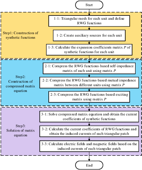
Figure 6: Algorithm flowchart of SBFM for solving array structures.

For a periodic array composed of B elements, the compressed matrix equation of SBFM is shown in Fig. 7, where W${}_{b\mathit{}b}$ represents the compressed self-impedance matrix of unit b, W${}_{p\mathit{}q}$ represents the compressed mutual-impedance matrix between unit p and unit q, and G${}_b$stands for the compressed exciting matrix of unit b.

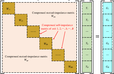
Figure 7: Schematic diagram of the matrix equation of SBFM for array structures.

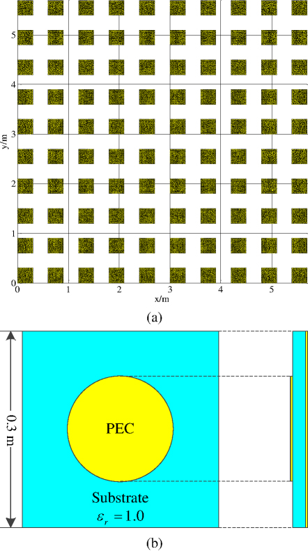
Figure 8: A 10$\times$10 circular microstrip patch antenna array: (a) layout of the array and (b) structure of a single unit.

The matrices in Fig. 7 can be computed as:

$$\{\begin{array}{c}{W}_{bb}=P_b^{\mathrm{H}}{Z}_{bb}{P}_b\hfill \\ W_{pq}=P_p^{\mathrm{H}}{Z}_{pq}{P}_q\hfill \\ G_b=P_b^{\mathrm{H}}{V}_b\hfill \end{array},$$

(24)

where P${}_{\mathrm{b}}$ is the expansion coefficients matrix of SFs, and Z${}_{b\mathit{}b}$ and V${}_b$ are impedance matrix and exciting matrix of MoM.

In the case of periodic structures, to obtain the expansion coefficients matrix of SFs defined on each unit (steps 1-3 in Fig. 6), QR decomposition can be used to extract the independent items from the solution space. Moreover, this may bring benefits such as using less SFs to get a satisfying accuracy. To further validate this, a 10$\times$10 circular microstrip patch antenna array is analyzed, as shown in Fig. 8.

Incident wave is a plane wave coming from +z axis and polarizing +x axis. Frequency of incident wave is 1.0 GHz. After triangulation, there are 100 units in the array and 628 RWG functions are defined on each unit. Thus, for the whole array, there are 62800 unknowns. Denote the distance between adjacent units by d and two cases are considered here: d=0.5$\lambda$ and d=1.0$\lambda$ ($\lambda$ is the wavelength of the incident wave).

Bistatic RCS of the antenna array on xoz plane and current coefficients of RWG functions are calculated using MoM, SBFM+SVD, and SBFM+QR. To evaluate the accuracy of different methods, the mean error of RCS and relative residual error of current coefficients are calculated here. They are defined as equations (26) and (27), respectively:

$${\delta }_{\mathrm{RCS}}=\frac{1}{N}\sum _{i=1}^N|{\sigma }_i^{\mathrm{SBFM}}-{\sigma }_i^{\mathrm{MoM}}|,$$

(25)

where $\sigma$${}_i$ represents the i-th data of BiRCS and N stands for the total number of data taken into consideration:

$${\delta }_I=\frac{||I_{\mathrm{SBFM}}-I_{\mathrm{MoM}}||}{||I_{\mathrm{MoM}}||},$$

(26)

where ||X|| represents the 2-norm of vector X.

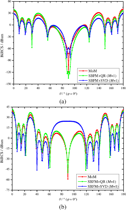
Figure 9: BiRCS on xoz plane: (a) d=0.5$\lambda$ and (b) d=1.0$\lambda$.

Figure 9 shows BiRCS data of the antenna array, from which we can see that the results of SBFM+QR are closer to MoM than SBFM+SVD if only one SF is adopted.

To be more specific, Fig. 10 exhibits the convergent curves of $\delta$${}_I$ changing with the number of SFs. In general, the accuracy of SBFM+SVD and SBFM+QR both improve with the growth of the number of SFs. However, there is a low point in SBFM+QR at M=1 in contrast to SBFM+SVD. This verifies our previous prediction: QR is better than SVD in the case of periodic arrays if only one SF is adopted. Furthermore, in terms of the fluctuation on convergent curves, QR is also less than SVD.

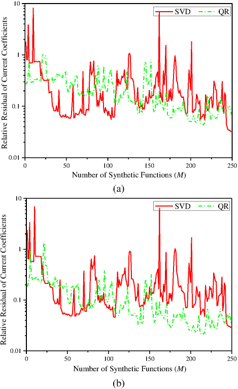
Figure 10: Relative residual error of current coefficients changing with the number of SFs: (a) $\mathrm{d}=0.5\lambda$ and (b) $\mathrm{d}=1.0\lambda$.

Table 2 shows the computational accuracy between different matrix decomposition methods. Interestingly, the accuracy of SBFM+QR at M=1 is approximately equal to SBFM+SVD at M=125 in terms of BiRCS. However, when it comes to current coefficients, accuracy of the former is apparently higher than the latter. This is easy to explain: RCS is an integral of all surface currents and accuracy is mainly determined by these strong currents. Thus, to get the same level of accuracy, $\delta$${}_I$ usually needs more SFs than $\delta$${}_{RCS}$. Table 3 exhibits the elapsed time and memory cost of different methods. From the comparison between SBFM+SVD and SBFM+QR, it is not difficult to see that the decrease of the number of SFs is meaningful.

Table 2: Computational accuracy of different matrix decomposition methods

	$\mathit{\delta }$${}_I$	$\mathit{\delta }$${}_{RCS}$
	0.5$\lambda$	1.0$\lambda$	0.5$\lambda$	1.0$\lambda$
SBFM+SVD	M=1	1.80	2.40	12.5	18.7
M=125	0.99	0.85	4.51	3.11
SBFM+QR	M=1	0.27	0.18	4.31	4.46

Table 3: Elapsed time and memory cost of SBFM and MoM

	P	Z	I	Total Time
MoM	0 s	3.16 h	53.76 h	56.94 h
	104.87 GB
SBFM + SVD	M=1	4.89 s	2.07 h	0.02 s	2.10 h
	273.02 KB
M=125	5.09 s	2.35 h	989.59 s	2.69 h
	4.16 GB
SBFM + QR	M=1	2.92 s	2.07 h	0.02 s	2.10 h
	279.86 KB

IV. CONCLUSION

SBFM and its application in periodic structures is discussed in this work. Unlike the traditional case of SVD decomposition, QR decomposition is used to extract expansion coefficients of SFs from solution space. Based on theoretical analysis, we prove that SBFM+QR can get the same level of accuracy with MoM with only one SF when a single body is concerned. Moreover, this feature can be extended to periodic arrays. For periodic arrays, only one synthetic function is enough to get high accuracy if SBFM+QR is adopted and this may lead to a series of benefits such as decreasing memory cost and improving efficiency.

ACKNOWLEDGMENT

This work was supported by the National Natural Science Foundation of China under Grant 62101564 and Hunan Provincial Natural Science Foundation of China under Grant 2022JJ20045.

REFERENCES

[1] R. Liu, G. Xiao, and Y. Hu, “Solving surface-volume integral equations for PEC and inhomogeneous/anisotropic materials with multibranch basis functions,” Applied Computational Electromagnetics Society (ACES) Journal, vol. 39, no. 2, pp. 108-114, 2024.

[2] W. Lu, W. Xiang, W. Wu, and W Yang, “The fast algorithms for electromagnetic analysis of the large-scale and finite periodic structures,” Chinese Journal of Radio Science, vol. 35, no. 1, pp. 85-92, 2020.

[3] W. He, Z. Yang, X. Huang, W. Wang, M. Yang, and X. Sheng, “Solving electromagnetic scattering problems with tens of billions of unknowns using GPU accelerated massively parallel MLFMA,” IEEE Trans. Antennas Propag., vol. 70, no. 7, pp. 5672-5682, 2022.

[4] C. Wu, L. Guan, P. Gu, and R. Chen, “Application of parallel CM-MLFMA method to the analysis of array structures,” IEEE Trans. Antennas Propag., vol. 69, no. 9, pp. 6116-6121, 2021.

[5] M. Li, T. Su, and R. Chen, “Equivalence principle algorithm with body of revolution equivalence surface for the modeling of large multiscale structures,” IEEE Trans. Antennas Propag., vol. 64, no. 5, pp. 1818-1828, 2016.

[6] M. Yang, B. Wu, X. Huang, and X. Sheng, “The progress of domain decomposition methods for 3D electromagnetic scattering problems,” Chinese Journal of Radio Science, vol. 35, no. 1, pp. 37-45, 2020.

[7] R. Zhao, Y. Chen, X. Gu, Z. Huang, H. Bagci, and J. Hu, “A local coupling multitrace domain decomposition method for electromagnetic scattering from multilayered dielectric objects,” IEEE Trans. Antennas Propag., vol. 68, no. 10, pp. 7099-7108, 2020.

[8] K. Fan, B. Wei, J. Chen, and B. He. “A spatial modes filtering FETD method combined with domain decomposition for simulating fine electromagnetic structures,” IEEE Microwave and Wireless Components Letters, vol. 32, no. 11, pp. 1259-1262, 2022.

[9] M. Li, M. A. Francavilla, R. Chen, and G. Vecchi, “Wideband fast kernel-independent modeling of large multiscale structures via nested equivalent source approximation,” IEEE Trans. Antennas Propag., vol. 63, no. 5, pp. 2122-2134, 2015.

[10] Y. Xu, H. Yang, R. Shen, L. Zhu, and X. Huang, “Scattering analysis of multiobject electromagnetic systems using stepwise method of moment,” IEEE Trans. Antennas Propag., vol. 67, no. 3, pp. 1740-1747, 2019.

[11] L. Matekovits, G. Vecchi, G. Dassano, and M. Orefice, “Synthetic function analysis of large printed structures: the solution space sampling approach,” IEEE Antennas Propag. Society International Symposium, no. 2, pp. 568-571,2001.

[12] L. Matekovits, V. A. Laza, and G. Vecchi, “Analysis of large complex structures with the synthetic-functions approach,” IEEE Trans. Antennas Propag., vol. 55, no. 9, pp. 2509-2521, 2007.

[13] H. Yuan, S. Gong, Y. Guan, and D. Su, “Scattering analysis of the large array antennas using the synthetic basis function method,” Journal of Electromagnetic Waves and Applications, vol. 23, pp. 309-320, 2009.

[14] B. Zhang, G. Xiao, J. Mao, and Y. Wang, “Analyzing large-scale non-periodic arrays with synthetic basis functions,” IEEE Trans. Antennas Propag., vol. 58, no. 11, pp. 3576-3584, 2010.

[15] W. Chen, G. Xiao, S. Xiang, and J. Mao, “A note on the construction of synthetic basis functions for antenna arrays,” IEEE Trans. Antennas Propag., vol. 60, no. 7, pp. 3509-3512, 2012.

[16] Y. Xu, H. Yang, and W. Yu, “Scattering analysis of periodic composite metallic and dielectric structures with synthetic basis functions,” Applied Computational Electromagnetics (ACES) Society Journal, vol. 30, no. 10, pp. 1059-1067,2015.

[17] Y. Xu, H. Yang, W. Yu, and J. Zhu, “An automatic scheme for synthetic basis functions method,” IEEE Trans. Antennas Propag., vol. 66, no. 3, pp. 1601-1606, 2018.

[18] Y. Xu, X. Huang, C. Liu, S. Zha, and J. Liu, “Synthetic functions expansion: automation, reuse, and parallel,” IEEE Trans. Antennas Propag., vol. 69, no. 3, pp. 1825-1830, 2021.

[19] N. Hu, Y. Xu, and P. Liu, “A numerical analysis of conformal energy selective surface array with synthetic functions expansion,” Applied Computational Electromagnetics Society (ACES) Journal, vol. 39, no. 2, pp. 115-122, 2024.

[20] Y. Xu, C. Liu, Z. Wu, N. Hu, J. Liu, and P. Liu, “Fast electromagnetic simulation method for large-scale quasi-periodic arrays,” Sci. Sin. Inform., vol. 54, no. 2, pp. 430-448, 2024.

[21] W. Lu, T. Cui, Z. Qian, X. Yin, and W. Hong, “Accurate analysis of large-scale periodic structures using an efficient sub-entire-domain basis function method,” IEEE Trans. Antennas Propag., vol. 52, no. 11, pp. 3078-3085, 2004.

[22] V. V. S. Prakash and R. Mittra, “Characteristic basis function method: A new technique for efficient solution of method of moments matrix equations,” Microwave and Optical Technology Letters, vol. 36, no. 2, pp. 95-100, 2003.

[23] C. S. Park, I. P. Hong, Y. J. Kim, and J. G. Yook, “Acceleration of multilevel characteristic basis function method by multilevel multipole approach,” IEEE Trans. Antennas Propag., vol. 68, no. 10, pp. 7109-7120, 2020.

[24] Y. Xu, H. Yang, J. Lu, W. Yu, W. Yin, and D. Peng, “Improved synthetic basis functions method for nonperiodic scaling structures with arbitrary spatial attitudes,” IEEE Trans. Antennas Propag., vol. 65, no. 9, pp. 4728-4741, 2017.

[25] Z. Wu, Y. Xu, P. Liu, T. Tian, and M. Lin, “An ultra-broadband energy selective surface design method: From filter circuits to metamaterials,” IEEE Trans. Antennas Propag., vol. 71, no. 7, pp. 5865-5873, 2023.

BIOGRAPHIES

Yanlin Xu received the B.S., M.S., and Ph.D. degrees in electronic science and technology from the National University of Defense Technology (NUDT), Changsha, China, in 2013, 2015, and 2018, respectively. He is currently an Associate Professor with the College of Electronic Science and Technology, NUDT. His current research interests include electromagnetic compatibility and protection, and computational electromagnetism.

Ning Hu (corresponding author) received the B.S. degree in electronic engineering and the M.S. degree in electronic science and technology from National University of Defense Technology (NUDT), Changsha, Hunan, P. R. China, in 2017 and 2019, respectively. He received the Ph.D. degree in information and communication engineering from NUDT in 2023. His research interests include electromagnetic compatibility and protection, and metamaterials and antennas.

Chenxi Liu (corresponding author) received the B.S. degree in electrical engineering and the M.S. and Ph.D. degrees in electronic science and technology from the National University of Defense Technology, Changsha, China, in 2013, 2015, and 2019, respectively. He is currently an Associate Professor with the College of Electronic Science, National University of Defense Technology. His research areas of interest include electromagnetically induced transparency analogy based on metamaterial and tunable metamaterials based on active components.

Hao Ding received the B.S. and M.S. degrees from Air Force Engineering University (AFEU), Xian, China, in 2013 and 2016, respectively, and the Ph.D. degree from the University and Institute of Microelectronics, Chinese Academy of Sciences (IMECAS), Beijing, China, and AFEU, in 2020. He is now working as a Lecturer with the National University of Defense Technology, Changsha, China. His research interests include IC and microsystem designs for electromagnetic compatibility and protection.

Jun Li received the M.S. degree from the National University of Defense Technology (NUDT), Changsha, China, in 2015. He is currently a senior engineer with the second representative office of Changsha area. His current research interests include electromagnetic compatibility antenna, and big data analysis.

ACES JOURNAL, Vol. 40, No. 2, 156–164
doi: 10.13052/2025.ACES.J.400209
© 2025 River Publishers

ABSTRACT

I. INTRODUCTION

II. THEORY AND PHENOMENON

III. EXPLANATION AND EXPANSION

IV. CONCLUSION

ACKNOWLEDGMENT

REFERENCES

BIOGRAPHIES