Analysis of Moving Bodies with a Direct Finite Difference Time Domain Method

Mohammad Marvasti and Halim Boutayeb

Department of Electrical Engineering
University of Quebec in Outaouais, Gatineau, Canada, J8X 3X7
halim.boutayeb@uqo.ca

Submitted On: June 23, 2023; Accepted On: December 6, 2023

ABSTRACT

This paper proposes an original and thorough analysis of the behavior of electromagnetic waves in the presence of moving bodies by using the finite difference time domain (FDTD) method. Movements are implemented by changing positions of the objects at each time step, through the classical FDTD time loop. This technique is suitable for non-relativistic speeds, thus for most encountered problems in antennas and propagation domain. The numerical aspects that need to be considered are studied. Then, different bodies in motion are examined: plane wave source with matching resistors, observation point, inclined partially reflecting surface (PRS), line source, and metallic cylinder illuminated by a plane wave. The results are compared with those of special relativity which are considered as the references. Some aspects of special relativity are present in the direct FDTD approach, such as the independence of the velocity of electromagnetic wave propagation with the speed of the source and Lorentz local time (with a different physical interpretation). It is shown that the amplitude of the electric field for a moving plane wave source does not increase with the speed of motion, if the impedance of the source is small. Moreover, for a moving scattering metallic wire, one can observe a phenomenon similar to shock waves.

Keywords: Doppler effect, electromagnetic theory, FDTD method, numerical analysis.

I. INTRODUCTION

The main laws of electromagnetism are contained in Maxwell’s equations. The finite difference time domain (FDTD) method is a rigorous and powerful tool for modeling electromagnetic devices. FDTD solves Maxwell’s equations directly without any physical approximation, and the maximum problem size is limited only by the extent of the computing power available. The FDTD method is based on the discretization of Maxwell’s equations in time and space domains. Invented in 1966 [1], it is applied for the first time in 1975 to study the effect of electromagnetic radiation on human eyes [2]. A microstrip patch antenna is analyzed in time domain in 1989, by using FDTD [3]. In 1990, the FDTD technique is used for the first time for microwave circuits [4]. In 1991, an algorithm is proposed to obtain the electromagnetic radiation in far field from near field results, in FDTD code [5]. Today, the FDTD method is used in a wide range of applications from DC to optics.

The problem of the interaction of electromagnetic waves with moving bodies has been an important subject of interest for a long time, due to its wide application in many domains such as radio sciences, optics, and astrophysics. Numerous investigations have been carried out in this area, which is interesting from a practical and theoretical point of view.

In the microwave domain, the study of electromagnetic problems with moving media is useful in many applications such as radar systems for the detection of vital signs [6, 7] or time-varying waveguides [8]. Time varying waveguides have been proposed for designing new RF devices such as magnet-less circulators or harmonic-free mixers [9-13].

In [14], the authors present a method based on the concept of propagators for analyzing the reflection and transmission of obliquely incident electromagnetic waves by a moving slab. The proposed propagators map the total field at any point inside the slab to the fields on the left-hand side boundary of the slab. In [15], Voigt-Lorentz transformations are used to obtain formulas for the intensity of the reflected and transmitted waves when electromagnetic radiation is incident on a moving dielectric slab. In [16], the reflection and transmission of a plane wave, with its electric vector polarized in the plane of incidence by a moving dielectric slab, are investigated theoretically. Two cases of movement are considered: the dielectric slab moves parallel to the interface, or the dielectric slab, moves perpendicular to the interface. In [17], the problem of the propagation of modes along a moving dielectric interface is considered, using a moving dielectric slab or a moving dielectric circular cylinder. In [18], the reflection of electromagnetic waves from a moving dielectric half-space is investigated for parallel and perpendicular motions of a dielectric medium. The paper [19] deals with the scattering of electromagnetic waves from a moving dielectric cylinder illuminated by a plane wave, by using the three-dimensional finite element method (FEM).

The FDTD method has been used by several authors for analyzing electromagnetic problems with moving bodies [20-29]. In [22-29], the authors propose a technique based on the integration Voigt-Lorentz transformations in FDTD. The main challenges of such an approach are to implement a relative time in a full-wave simulator and to consider complex problems with, for example, multiple bodies moving at different speeds.

In this paper, continuing our previous work [30], we assess the effectiveness of a direct FDTD approach where the implementation of movements is done by changing the positions of bodies at each cycle of the FDTD time loop. With this “brute-force” approach, time is implicitly absolute, and Voigt-Lorentz transformations are not implemented. This technique is suitable for non-relativistic electromagnetic problems with moving bodies, thus for most encountered electromagnetic problems.

The numerical aspects that need to be considered in the proposed approach are studied in detail. Then, different problems are investigated: moving plane wave source with matching resistors, moving observation point, moving inclined partially reflecting surface (PRS), moving line source, and moving metallic cylinder illuminated by a plane wave. The results, in terms of Doppler frequency shift and changes in amplitude of the electric field, are compared with those of special relativity, which are considered as the references. Some aspects of special relativity are present in the direct FDTD approach, such as the independence of the velocity of electromagnetic wave propagation with the speed of the source and Lorentz local time (with a different physical interpretation). Some of the obtained results agree with special relativity. Other ones are different, but the differences are negligible for non-relativistic speeds. The results obtained with our analysis give new physical insights into the propagation of waves with moving bodies. In particular, it is shown that the amplitude of the electric field for a moving plane wave source does not increase with the speed of motion, if the impedance of the source is small. Moreover, for a moving scattering metallic wire, one can observe a phenomenon similar to shock waves. In the literature, electromagnetic shock waves were analyzed in different contexts, such as gyromagnetic media and non-linear transmission lines [31-33].

The remainder of the paper is organized as follows. Section 2 presents numerical aspects that need to be taken into account. Section 3 shows the study of the frequency shift and amplitude variation of the electric field in time and frequency domains for a moving plane wave source. A moving observation point is considered in Section 4. Section 5 deals with the illumination by a plane wave of a moving partially reflecting surface (PRS) with different angles of inclination of the PRS. Problems with moving line source and moving metallic wire are considered in Section 6. Concluding remarks are given in Section 7.

II. ANALYSIS OF THE NUMERICAL ASPECTS

A. Type of excitation

For better analysis and detection of the frequency variation due to the Doppler effect, we consider as the exciting source a windowed sine signal $E_i(t)=\mathrm{\Pi }(\frac{f_0}{N}t)\sin (2\pi f_{0}t)$, presenting a modulated sinusoid $E_i(f)=\frac{N}{f_0}\mathrm{Sinc}(\frac{f\text{-}{f}_0}{N{f}_0})$ spectrum, where $f_0$ is the frequency of excitation and $N$ is the number of periods of sine function considered for simulation. This excitation provides a sharp frequency spectrum and makes frequency identification accurate and simple.

B. Dispersion and stability

For simplicity, in the paper, we consider the same space mesh in all axes, ${\delta }_x={\delta }_y={\delta }_z$. Due to numerical dispersion, the phase velocity of the wave changes with the angle in the computational volume [34]. This effect decreases by reducing the size of the space mesh. For example with ${\delta }_x=\frac{\lambda }{40}$ the maximum of velocity change is about $0.05\%$ [34].

The dispersion equation and the stability criterion are the same as those calculated without motion, for the problems considered in this paper (moving source, moving observer, and moving scatterers). Different dispersion equations and stability criteria would be required if the field is moved, but this problem is not considered here. The FDTD dispersion equation for a plane wave propagating in the $x$-axis can be written

$$\omega =\frac{2}{{\delta }_t}\arcsin \left(\frac{c{\delta }_t}{{\delta }_x}\sin \left(\frac{k{\delta }_x}{2}\right)\right),$$

(1)

where $\omega$ is pulsation frequency, ${\delta }_t$ is time step, $c$ is the speed of light in vacuum, and $k$ is the propagation constant. Figure 1 shows the dispersion diagram for different values of space mesh. In next subsection, the propriety of the dispersion diagram is used to make undesirable waves having high frequencies propagate with lower speed than desirable waves, for better differentiation.

Figure 1: Numerical dispersion for different values of ${\delta }_x$.

C. Effect of discontinuous motion and its mitigation

Let us consider a plane wave source parallel to $zoy$ plane and moving in $x$ direction. The plane wave source is constituted of $z$-polarized electric current sources. Due to the discretization in the classical FDTD numerical method, the source location doesn’t change continuously because it doesn’t move inside a cell. Instead, in the FDTD code, for a specific value of source motion speed $v$, the position of the source is fixed for $n{\delta }_t$ with $n=\lfloor \frac{{\delta }_x}{v{\delta }_t}\rfloor$. $\lfloor \text{.}\rfloor$ stands for floor function. ${\delta }_t$ and ${\delta }_x$ are the time step and space mesh. Then, after this time, the source moves one cell in the desired direction. Figure 2 illustrates the discontinuous movement of the source in FDTD, the ideal continuous motion, and an approximate model for the discontinuous movement.

Figure 2: Discontinuous movement of plane wave source.

Without motion, the time-domain signal received from a plane wave can be written

$$E(t)=\exp (\text{-}j(kx+\omega t)).$$

(2)

As shown Fig. 2, the position of the source can be approximated by using a sine function

$$x_p(t)=x_0+vt+a\sin ({\omega }_{\mathrm{d}}t),$$

(3)

where $a=\frac{{\delta }_x}{2}$ and ${\omega }_{\mathrm{d}}=\frac{2\pi }{{\delta }_t\lfloor \frac{{\delta }_x}{v{\delta }_t}\rfloor }$ . Because of the additional term $a\sin ({\omega }_{\mathrm{d}}t)$, the time-domain signal received for the moving plane wave source can be written

$$E^{\prime \prime }(t)=E^{\prime }(t)\exp (\text{-}j(ka\sin ({\omega }_{\mathrm{d}}t))),$$

(4)

where $E^{\prime }(t)$ is the signal received by observer if the source moves continuously. We can expand (4) by using the Fourier series

$E^{\prime \prime }(t)$	$=E^{\prime }(t){\displaystyle \sum _{n=\text{-}\mathrm{\infty }}^{\mathrm{\infty }}}{c}_n\exp (jn{\omega }_{\mathrm{d}}t),$	(5)
$c_n$	$={\displaystyle \frac{{\omega }_{\mathrm{d}}}{2\pi }}{\displaystyle {\int }_{\text{-}\frac{\pi }{{\omega }_{\mathrm{d}}}}^{\frac{\pi }{{\omega }_{\mathrm{d}}}}}{e}^{\text{-}j(ka\sin ({\omega }_{\mathrm{d}}t))}{e}^{\text{-}jn{\omega }_{\mathrm{d}}t}\mathit{d}t.$	(6)

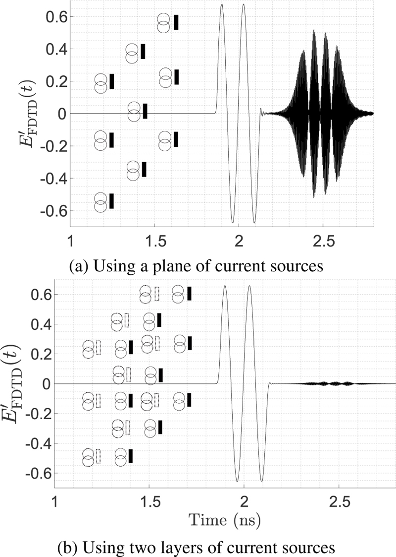
Figure 3: Observed signal in time domain for a moving plane wave source in FDTD. Using two layers for the plane wave source can mitigate the undesirable effects due to discontinuous motion.

With a change of variable $t^{\prime }={\omega }_{\mathrm{d}}t$, the coefficients $c_n$ can be written

$$c_n=\frac{1}{2\pi }{\int }_{-\pi }^{\pi }{e}^{\text{-}j(ka\sin (t^{\prime }))}{e}^{\text{-}jn{t}^{\prime }}\mathit{d}{t}^{\prime }.$$

(7)

By using the definition of the Bessel function of the first kind, equation (5) can be expressed as

$$E^{\prime \prime }(t)=E^{\prime }(t)\sum _{n=\text{-}\mathrm{\infty }}^{\mathrm{\infty }}{\mathrm{J}}_n(ka)\exp (jn{\omega }_{\mathrm{d}}t).$$

(8)

This shows that the received signal contains $E^{\prime }(t)$ and other waves that are made from the modulation of $E^{\prime }(t)$ with center frequencies of $n{\omega }_{\mathrm{d}}$, $n=1,2,\mathrm{\dots }$.

The FDTD simulations confirm our analysis, as shown in Fig. 3 (a), where the windowed sine signal is the expected signal for continuous motion, and the high frequency modulated signal is due to the discontinuous motion effect. In this figure, we were able to separate undesirable signals from the expected signal by using the FDTD dispersion equation such that the waves at higher frequencies propagate with less speed.

We propose now a technique to mitigate the undesirable effects. By using a second layer of current sources to make the plane wave source, we can show that the discontinuous motion adds the term $a\sin ({\omega }_{\mathrm{d}}t)+a\sin ({\omega }_{\mathrm{d}}t+\pi )=a\sin ({\omega }_{\mathrm{d}}t)$ - $a\sin ({\omega }_{\mathrm{d}}t)=0$. Thus, this method can suppress the undesirable effects. FDTD simulations, as shown in Fig. 3 (b), confirm that by using two layers of current sources, the undesirable effects are mitigated. The same phenomena have been observed by using a moving PRS, whose thickness needs to be at least one cell in order to mitigate the undesirable effects.

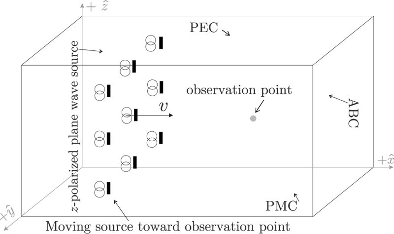
Figure 4: Plane wave source moving toward the observer.

D. Space mesh and time step

Because of the discontinuous motion in FDTD, as illustrated in Fig. 2, the space mesh needs to be sufficiently small to detect the smallest velocity considered in a problem. The pulsation frequency ${\omega }_{\mathrm{d}}$ needs to be larger than the maximum pulsation frequency considered, ${\omega }_{\max }$. Based on empirical analysis,

$${\omega }_{\mathrm{d}}>2{\omega }_{\max }.$$

(9)

After simplification, we can show that the following condition is required:

$${\delta }_x<0.5\frac{v}{f_{\max }},$$

(10)

where $f_{\max }$ is the maximum frequency considered. From this equation, if the speed $v$ is decreased, ${\delta }_x$ must be decreased. The time step needs also to be reduced because of the classical stability criterion ${\delta }_t<\frac{{\delta }_x}{c\sqrt{3}}$.

III. MOVING PLANE WAVE SOURCE

A. Structure and definitions of the analyzed parameters

A plane wave source that is moving in $+\widehat{x}$ direction toward the observer with speed $v$, is considered, as shown in Fig. 4. Mur’s absorbing boundary conditions (ABCs) [35] are used in boundaries parallel to $zoy$ plane. Perfect magnetic conductors (PMCs) and perfect electric conductors (PECs) are used in other boundaries to model an infinite structure.

$E_z^{\prime }$ and $E_z$, are the electric field components in $z$-axis observed by the observation point for a moving source and for a source at rest, respectively. $f^{\prime }$ is the frequency of observed signals when the source is moving, and $f$ is the frequency when the source is at rest. $A_f^{\prime }$ and $A_t^{\prime }$ are the amplitudes of observed signals in the frequency and time domains, respectively, when the source is moving. $A_f$ and $A_t$ are the same amplitudes when the source is at rest.

B. Model of the plane wave source

Figure 5 presents the model of a realistic plane wave source in FDTD. It is made of $z$-polarized electric current sources and resistors with resistance $R$. A similar model has been used in [36, 37] for analyzing a Fabry-Perot cavity excited from its inside.

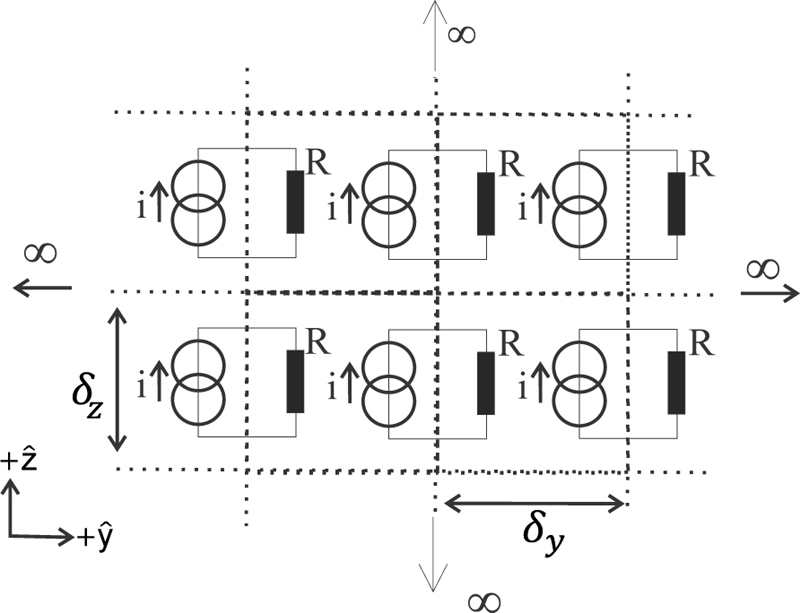
Figure 5: Model of a plane wave source used in FDTD.

C. Speed of wave propagation independent of the speed of the source

By using two observation points, one can measure the speed of propagation of the plane wave for different values of the speed of the plane wave source. It is confirmed that the speed of wave propagation in FDTD does not change when the source is moving. This shows that the direct FDTD method is in agreement with the following postulate from the special theory of relativity: “light is always propagated with a definite velocity $c$ which is independent of the state of motion of the emitting body”[38].

D. Doppler frequency shift and amplitude variation of electric field in frequency domain

An ideal source with low output impedance ($R$ is small) is considered. Figure 6 (a) shows the signal observed in the frequency domain at different normalized speeds of motion $\frac{v}{c}$. From these curves, the changes of the main frequency and of the amplitude at the main frequency due to motion are measured, as shown in Fig. 6 (b), and the curve-fitted results can be written as

$$\frac{f^{\prime }}{f}=\frac{A_f}{A_f^{\prime }}=\frac{1}{1\text{-}\frac{v}{c}}.$$

(11)

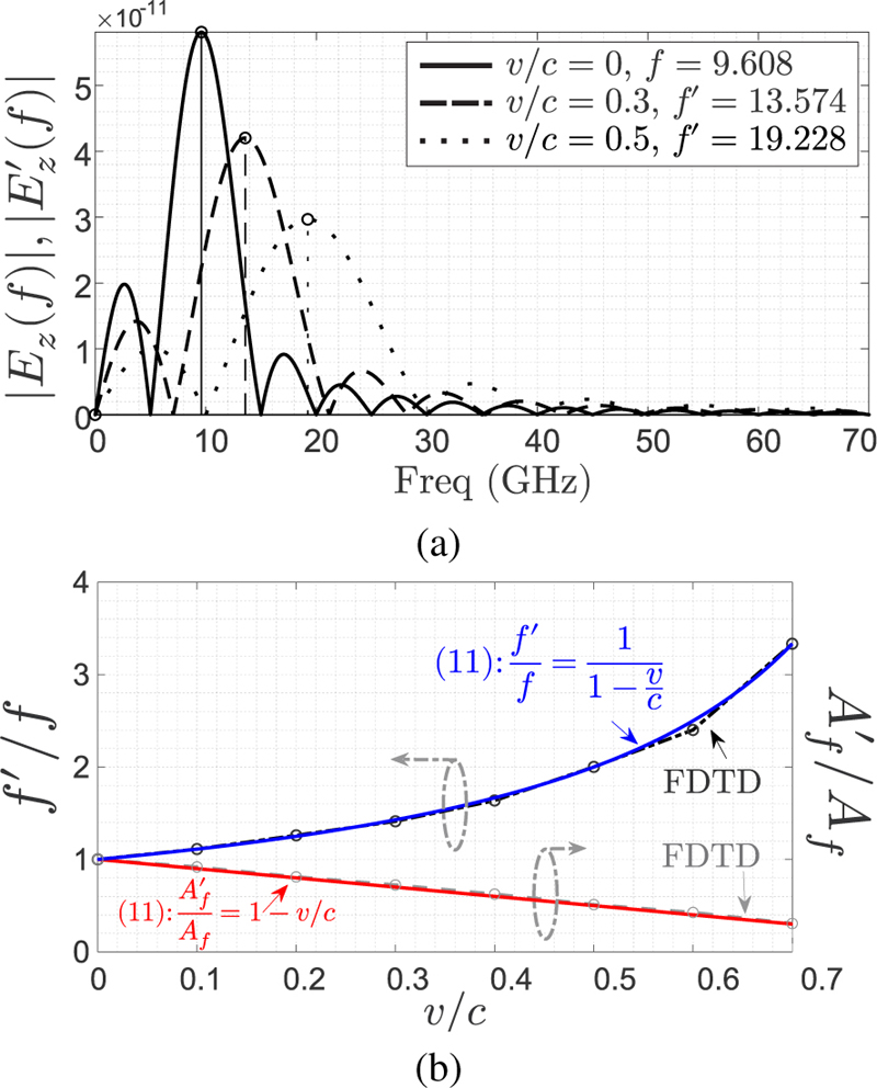
Figure 6: Simulated results for an ideal plane wave source moving with speed $v$ toward the observer: (a) Observed signal in the frequency domain for different values of $\frac{v}{c}$, (b) Doppler frequency shift and amplitude variation of the observed electric field in frequency domain versus $\frac{v}{c}$.

In special relativity, the Doppler effect formula for the moving source is given by $\frac{f^{\prime }}{f}={\gamma }^{\text{-}1}\frac{1}{1\text{-}\frac{v}{c}}$, where $\gamma =\frac{1}{\sqrt{1\text{-}{(\frac{v}{c})}^2}}$. A technique will be proposed later in order to take into account the relativistic effects.

E. Effect of the impedance of a plane wave source in motion

The amplitude of the signal in time domain does not change with the motion of the source if the output impedance of the source is small, as shown in Fig. 7 (a).

A high-impedance source can be modeled by using current sources without the resistors. For this case, Fig. 7 (b) shows that the amplitude of the signal in time domain increases with the speed of the source. The simulated results fit with the closed-form expression$\frac{A_t^{\prime }}{A_t}=\frac{1}{1\text{-}\frac{v}{c}}$.

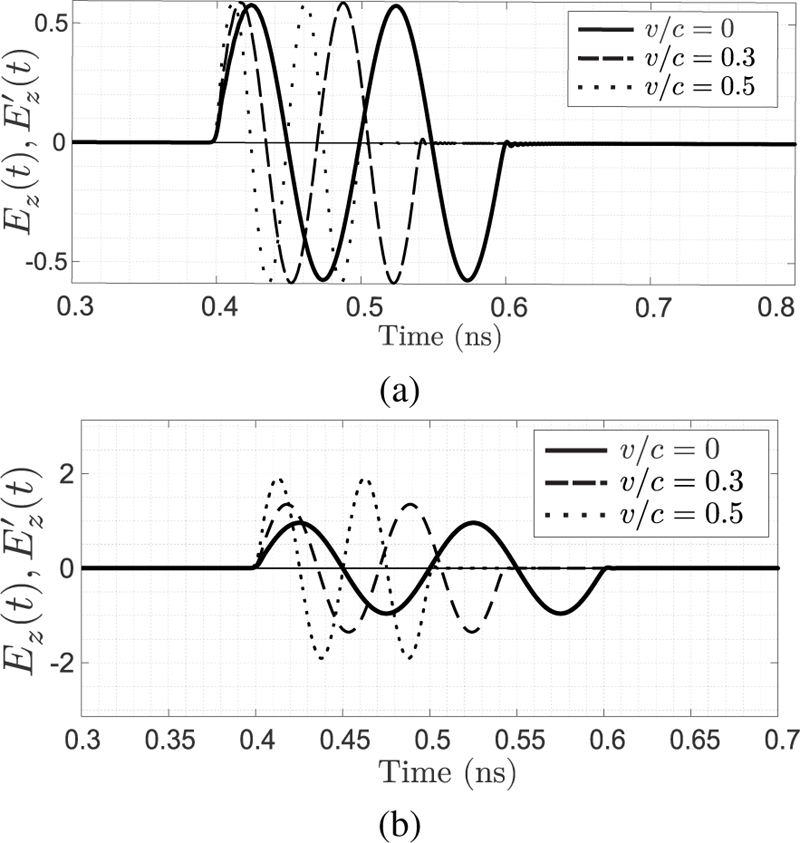
Figure 7: Simulated signal in time domain for plane wave source moving with speed $v$ toward observer, for different values of $\frac{v}{c}$: (a) Ideal plane wave source, (b) Plane wave source without resistors.

Based on the analysis presented in this subsection, it is suggested that previous studies on electromagnetism with moving objects should be revisited. For example, Heaviside derived from Maxwell’s equations the electric field of a moving charge, and he found that the amplitude of this electric field grows without bounds with $\frac{v}{c}$ [39]. At Heaviside’s time, this effect has been used as an argument against the possibility for a charge (or any object) to move at a speed greater than the speed of light. However, if the charge has a low output impedance, the amplitude of its electric field should not increase with the motion, as it has been shown in the present work.

F. Technique for implementing relativistic Doppler effect for moving source

The relativistic Doppler effect for the moving source can be obtained in the direct FDTD method, if the signal of the moving source is modified before its introduction in the FDTD time loop. This can be done by using the formula

$$E_{z,source\mathrm{\_}modif}(t)=E_{z,source}({\gamma }^{-1}t).$$

(12)

It is worth mentioning that, with the proposed approach, it is possible to consider multiple sources moving at different relativistic speeds.

IV. MOVING OBSERVATION POINT

A. Structure and definitions of the parameters

Let us consider an observation point moving in -$x$ direction (toward the source) with the speed $v$ as shown in Fig. 8.

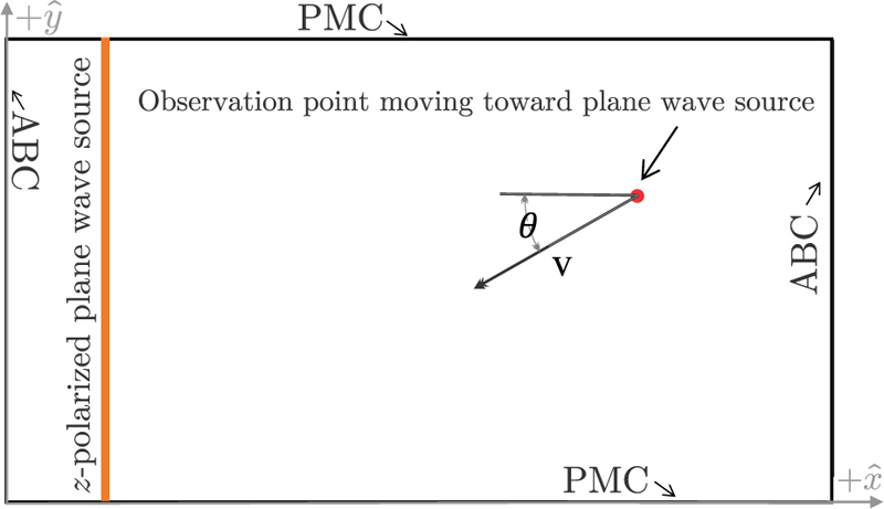
Figure 8: Observation point moving toward a plane wave source, in normal or oblique direction.

The observer measures $E_z^{\prime }$ and $E_z$, the electric field component in $z$-axis for moving observer and for observer at rest, respectively. We call $f^{\prime }$ the frequency of observed waves when the observation point is moving and $f$ the frequency when the observer is at rest. $A_f^{\prime }$ and $A_t^{\prime }$ are the amplitudes of observed waves in the frequency and time domains, respectively, when observer is moving. $A_f$ and $A_t$ are the same amplitudes when observer is at rest.

B. Time domain signal and Lorentz local time

Figure 9 shows the signal received by the observer in FDTD, in the time domain. One can note that the amplitude of the signal does not change with the motion, i.e, $\frac{A_t^{\prime }}{A_t}=1$. We also observe that

$$E_z^{\prime }(t)=E_z\left(t(1+\frac{v}{c})\right).$$

(13)

For example, for $t=0.34ns$ and $v/c=0.6$, we have $E_z^{\prime }(0.34)=E_z(0.34(1+0.6))=E_z(0.544)$. This has been verified for different values of $t$ and for different values of $v/c$. Equation (13) can be explained by the fact that if we replace $x$ with $x$-$vt$ in the phase of a plane wave $kx$-$\omega t$, we obtain $k(x$-$vt)$ - $\omega t=kx$-$\omega t(1+kv/\omega )=kx$-$\omega t(1+v/c)$, since $k/\omega =1/c$ for a plane wave propagating in free space.

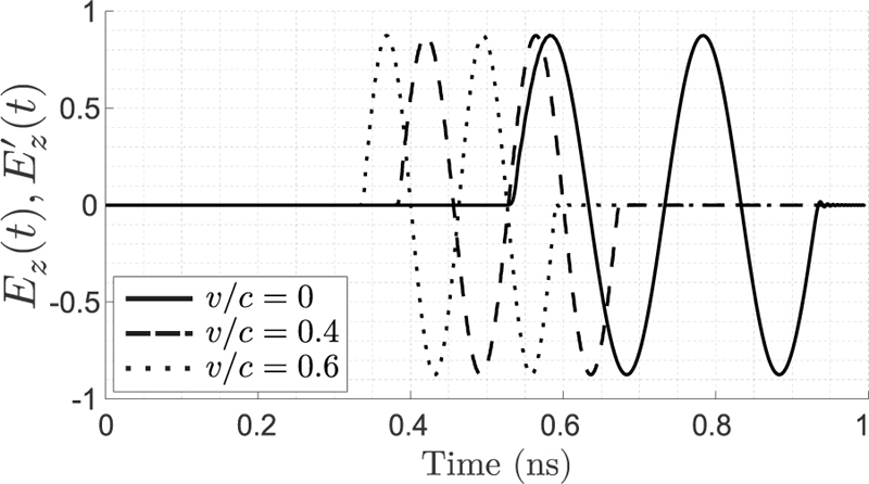
Figure 9: Simulated signal in time domain for observation point moving in normal direction toward -$x$ with speed $v$, for different values of $\frac{v}{c}$.

The parameter $t(1\pm v/c)$ of (13) has an analogy with Lorentz “local” time $t^{\prime }=t\pm xv/c^2$. Indeed $t(1\pm v/c)=t\pm tv/c=t\pm xv/c^2$. The last calculation is obtained by replacing the second $t$ with $x/c$.

The time parameter $t^{\prime }$ in Lorentz transformation is given by $t^{\prime }=\gamma (t\pm xv/c^2)$ [38]. In special relativity, this parameter $t^{\prime }$, which is often written $t^{\prime }=\gamma t(1\pm v/c)$, represents the true time for an observer in a moving frame. In the direct FDTD program, the term $\gamma$ is missing, and the parameter $t(1\pm v/c)$ represents the Doppler effect in time domain. Thus, Lorentz local time is present in the direct FDTD method but with a different physical interpretation.

C. Doppler frequency shift and amplitude of the electric field in frequency domain

Figure 10 shows the signal received by the observer in FDTD, in frequency domain. As shown in Fig. 11, the center frequency and the amplitude in frequency domain vary according to

$$\frac{f^{\prime }}{f}=\frac{A_f}{A_f^{\prime }}=1+\frac{v}{c}.$$

(14)

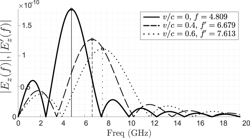
Figure 10: Simulated signal in frequency domain for observation point moving with speed $v$ toward -$x$ in normal direction, for different values of $\frac{v}{c}$.

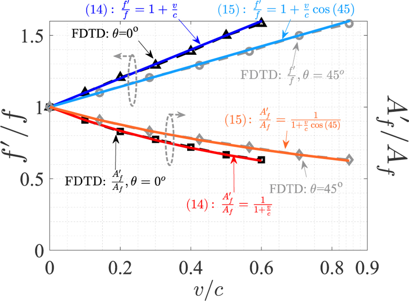
Figure 11: Simulated Doppler frequency shift and amplitude of the electric field in frequency domain for observation point moving with speed $v$ toward -$x$ in normal direction or at ${45}^{\circ }$, versus $\frac{v}{c}$.

In special relativity, the Doppler effect formula for the moving observer is given by $\frac{f^{\prime }}{f}=\gamma (1+\frac{v}{c})$. Based on the time domain results in the previous subsection, the change of amplitude in frequency domain can be understood by the relation $ℱ(g(|a|t))=\frac{1}{|a|}𝒢(\frac{f}{|a|})$, where $ℱ(\text{.})$ stands for Fourier transform operator, $𝒢(f)$ is Fourier transform function of a signal $g(t)$, and $a$ is a constant. In our case $a=1+\frac{v}{c}$.

From Fig. 10, it is interesting to note that $\int |E_z^{\prime }(f)|\mathit{d}f=\int |E_z(f)|\mathit{d}f=\mathrm{Constant}$ for anyvalue of $\frac{v}{c}$.

For motion in $+x$ direction (observer moving away from the source), in (14), one should replace $v$ with -$v$ (these cases were validated numerically).

D. Motion in oblique direction

We consider now that the observer is moving obliquely with the angle $\theta$ toward the source. The results are presented in Fig. 11. The changes of the frequency and of amplitude in frequency domain agree now with

$$\frac{f^{\prime }}{f}=\frac{A_f}{A_f^{\prime }}=1+\frac{v}{c}\cos \theta .$$

(15)

According to special relativity, we should have $\frac{f^{\prime }}{f}=\gamma (1+\frac{v}{c}\cos \theta )$. Again, the missing $\gamma$ factor can be omitted for non-relativistic speeds.

E. Technique for implementing relativistic Doppler effects for moving observer

The relativistic Doppler effect for the moving observer can be obtained in the direct FDTD method, if the observed signal is modified (post-processing), by using the following formula:

$$E_{z,obs\mathrm{\_}modif}(t)=E_{z,obs}(\gamma t).$$

(16)

V. MOVING PARTIALLY REFLECTING SURFACE

A. Straight PRS

A PRS that is parallel to the plane wave source is moving in -$x$ direction (toward the source), with the speed $v$. The observation point is between the source and the PRS, as shown in Fig. 12. FDTD simulations (Fig. 13) show that frequency can be written

$$\frac{f^{\prime }}{f}=\frac{1+\frac{v}{c}}{1\text{-}\frac{v}{c}}.$$

(17)

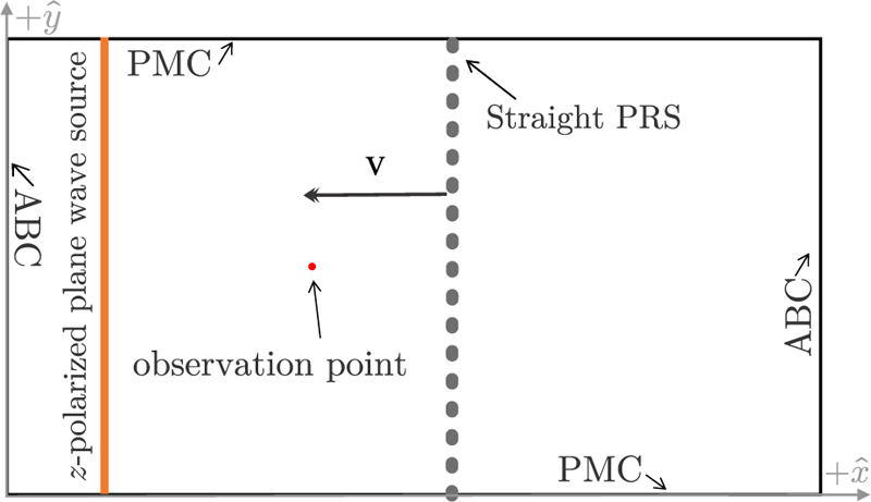
Figure 12: Straight PRS moving toward a plane wave source.

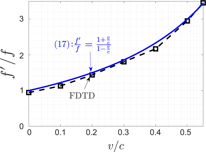
Figure 13: Simulated Doppler frequency shift for straight PRS moving in -$x$ direction (toward the source),versus $\frac{v}{c}$.

(17) can be understood as the combination of two Doppler effects: the frequency shift due to an observer (the PRS) moving toward the source (numerator part) and the frequency shift due to a source (the PRS acts as a source after diffracting the received field) moving toward the observer (denominator part). This formula is well known by radar engineers.

It is interesting to note that special relativity predicts the same formula (17) for a moving plane reflector with normal incidence. Thus, the direct FDTD method could be used for some problems at relativistic speeds.

B. Inclined PRS

The PRS is now inclined with the angle ${\theta }_{\mathrm{PRS}}$, and it is moving in -$x$ direction (toward the source), with the speed $v$ (Fig. 14). First, it is worth noting that a wave propagating at an angle $\theta$ in a frame moving with the speed $v$ will be seen in the stationary frame as propagating at the angle ${\alpha }_{\mathrm{B}}$, as given by Bradley’s aberration formula [40] (this formula has been validated with FDTD)

$${\alpha }_{\mathrm{B}}=\arctan \left(\frac{\sin (\theta )}{\cos (\theta )+\frac{v}{c}}\right).$$

(18)

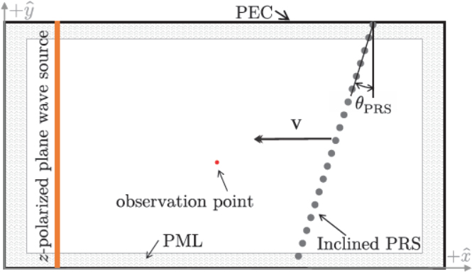
Figure 14: Inclined PRS moving toward a plane wave source.

For inclined PRS, a graphical method can be used to derive the Doppler effect formula, as illustrated in Fig. 15. From this figure, we obtain

$$\frac{f^{\prime }}{f}=\frac{\sin ({\theta }_{\mathrm{PRS}})}{\sin ({\alpha }_1\text{-}{\theta }_{\mathrm{PRS}})},$$

(19)

where ${\alpha }_1$ is the angle of the reflected wave, and it can be written

$${\alpha }_1=2\arctan \left(\frac{\tan ({\theta }_{\mathrm{PRS}})}{1+\frac{v}{c}}\right).$$

(20)

For a PRS moving in $+x$ direction (away from the source), the same formula (19) can be obtained, except that ${\alpha }_1$ should be replaced by

$${\alpha }_2=\pi -2\arctan \left(\frac{\tan ({\theta }_{\mathrm{PRS}})}{1-\frac{v}{c}}\right).$$

(21)

Good agreements are obtained between full-wave simulations and the proposed analytical formulas, as shown in Fig. 16. Numerical and analytical solutions for ${\alpha }_1$ and ${\alpha }_2$ are shown in Fig. 17, where we have also plotted ${\alpha }_B$ (for $\theta ={90}^{\circ }$) for comparison. Figure 18 shows how the different angles are measured accurately, with a numerical protractor.

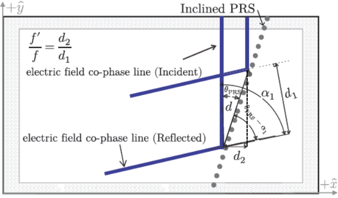
Figure 15: Graphical method for deriving the frequency of reflected wave for a moving inclined PRS.

Equation (19) is novel and simple to apply. The relativistic formula, which is given by $\frac{f^{\prime }}{f}=\frac{1+2\frac{v}{c}\cos ({\theta }_{\mathrm{PRS}})+{(\frac{v}{c})}^2}{1\text{-}{(\frac{v}{c})}^2}$, differs from the direct FDTD only for ${\theta }_{\mathrm{PRS}}\ne 0^{\circ }$ and relativistic speeds.

Figure 16: Simulated Doppler frequency shift for inclined PRS moving toward the source, for ${\theta }_{\mathrm{PRS}}={45}^{\circ }$ and ${25}^{\circ }$, versus $\frac{v}{c}$.

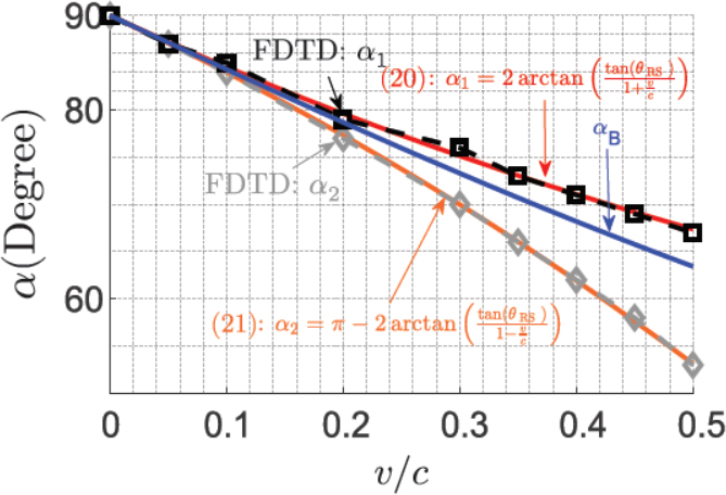
Figure 17: Simulated reflection angles for inclined PRS moving with speed $v$ toward $\pm x$ directions, with ${\theta }_{\mathrm{PRS}}={45}^{\circ }$. Bradley’s aberration angle ${\alpha }_B$ is also plotted for comparison.

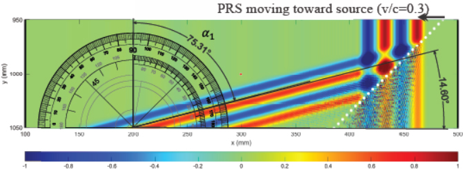
Figure 18: Illustration of the method used to measure the angle of reflected wave in FDTD simulations for a moving inclined PRS, with a numerical protractor. In this example, the PRS moves toward the source in -$x$ direction with $\frac{v}{c}=0.3$ and ${\theta }_{\mathrm{PRS}}={45}^{\circ }$. The measured angle gives ${\alpha }_1$ which is plotted versus $v/c$ in Fig. 17. One region part of the computational volume is shown, for better visualization.

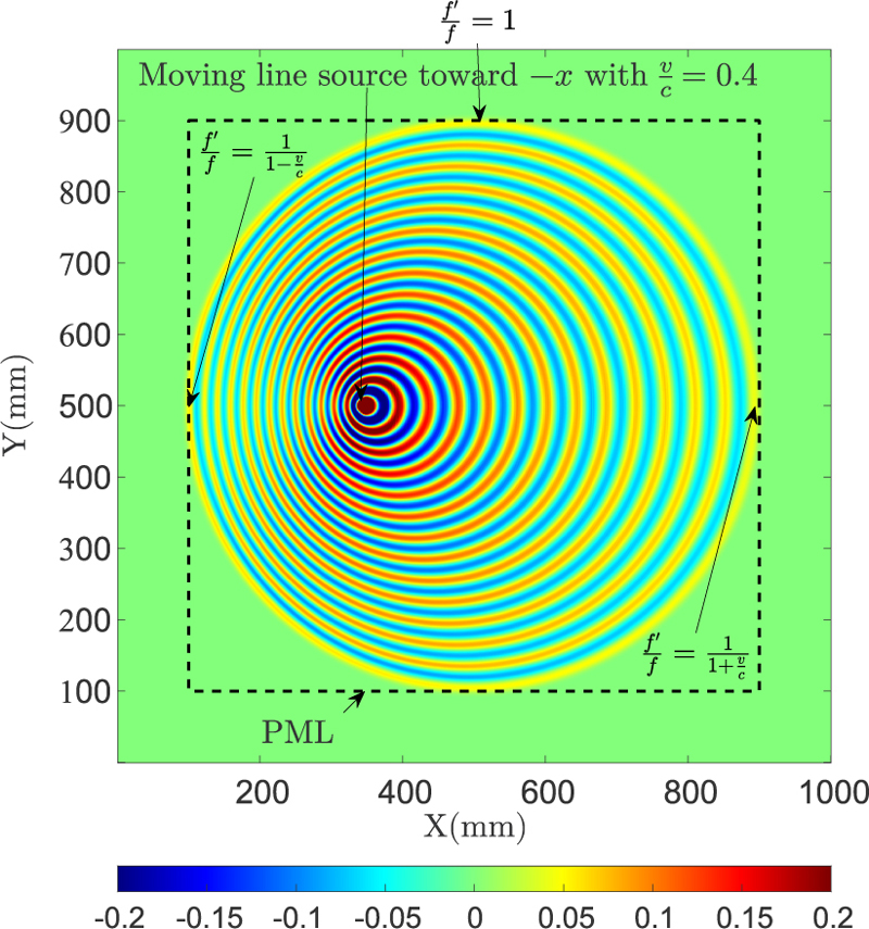
Figure 19: Electric field distribution for a line source moving toward -$x$ direction with $\frac{v}{c}=0.4$.

VI. MOVING LINE SOURCE AND METALLIC WIRE ILLUMINATED BY A PLANE WAVE

A. Moving line source

We consider a line source made of current sources and which generates a cylindrical wave when it is at rest. Figure 19 shows the electric field distribution at a time instant when the line source is in motion. By measuring the different wavelengths (i.e, distances between consecutive maxima) at the different directions, we obtain results for the Doppler effect that agree with the analysis of the plane wave source, as shown in Fig. 19.

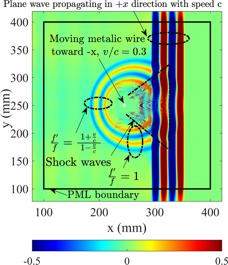
Figure 20: Electric field distribution for a metallic wire moving toward a plane wave source in -$x$ direction with $\frac{v}{c}=0.3$. The plane wave is propagating in $+x$ direction with speed $c$.

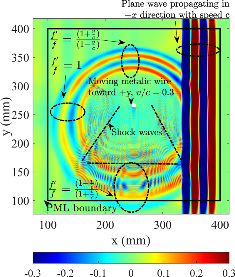
Figure 21: Electric field distribution for a metallic wire moving in $+y$ direction with $\frac{v}{c}=0.3$, and a plane wave propagating in $+x$ direction with speed $c$.

B. Moving metallic wire illuminated by a plane wave

A metallic wire is moving in -$x$ direction with speed $v$, and it is illuminated by a plane wave propagating in$+x$ direction, with speed $c$. Figure 20 shows the electric field distribution at a time instant. Based on the analysis of the wavelengths, the Doppler effect is indicated at different directions in Fig. 20. These results confirm the previous analysis on the plane reflector.

In Fig. 20, we can observe the presence of additional waves, which are highlighted in the back of the moving metallic wire in a region with triangular shape. Based on simulations not shown here, the time step and the cell size have no effect on these additional waves. We conclude that they are not due to numerical effects, but they are inherent to Maxwell’s equations. They can be associated with shock waves, due to their similarities with these types of waves. These waves can also be observed if the metallic wire moves in a direction perpendicular to the plane wave, as shown in Fig. 21. It should be noted that electromagnetic shock waves have been already observed in the literature but with other contexts, such as gyromagnetic media and non-linear transmission lines [31-33].

VII. CONCLUSION

In this paper, we propose a non-relativistic finite difference time domain method, and we assess the effectiveness of this technique by analyzing electromagnetic problems with different bodies in motion: plane wave source, line source, observer, partially reflecting surface and metallic wire. In the proposed direct FDTD method, movements are implemented by changing positions of the objects at different time instants, through the classical FDTD time loop.

First, the numerical aspects are analyzed thoroughly. Then, several analytical formulas for the Doppler frequency shifts, amplitudes of electric field and angles of reflection are derived, validated with full-wave simulations and compared with relativistic formulas (reference formulas). These results show that the direct FDTD method is suitable for non-relativistic speeds.

Furthermore, some aspects of special relativity are present in the direct FDTD approach, such as the independence of the velocity of electromagnetic wave propagation with the speed of the source and Lorentz local time (with a different physical interpretation). The results obtained with our analysis give new physical insights into the propagation of waves with moving bodies. For instance, it is shown that the amplitude of the electric field for a moving plane wave source does not increase with the speed of motion, if the impedance of the source is small. Moreover, electromagnetic shock waves can be observed in FDTD simulations of a metallic wire illuminated by a plane wave.

The proposed technique has the advantage of being simple to implement, and it can be used to consider, for non-relativistic speeds, multiple objects moving at different speeds, accelerating objects, or rotatingobjects.

REFERENCES

[1] K. Yee, “Numerical solution of initial boundary value problems involving Maxwell’s equations in isotropic media,” IEEE Transactions on Antennas and Propagation, vol. 14, no. 3, pp. 302-307,1966.

[2] A. Taflove and M. E. Brodwin, “Numerical solution of steady-state electromagnetic scattering problems using the time-dependent Maxwell’s equations,” IEEE Transactions on Microwave Theory and Techniques, vol. 23, no. 8, pp. 623-630,1975.

[3] A. Reineix and B. Jecko, “Analysis of microstrip patch antennas using finite difference time domain method,” IEEE Transactions on Antennas and Propagation, vol. 37, no. 11, pp. 1361-1369,1989.

[4] D. M. Sheen, S. M. Ali, M. D. Abouzahra, and J.-A. Kong, “Application of the three-dimensional finite-difference time-domain method to the analysis of planar microstrip circuits,” IEEE Transactions on Microwave Theory and Techniques, vol. 38, no. 7, pp. 849-857, 1990.

[5] K. S. Yee, D. Ingham, and K. Shlager, “Time-domain extrapolation to the far field based on FDTD calculations,” IEEE Transactions on Antennas and Propagation, vol. 39, no. 3, pp. 410-413, 1991.

[6] M. S. Rabbani, J. Churm, and A. P. Feresidis, “Fabry–Pérot beam scanning antenna for remote vital sign detection at 60 GHz,” IEEE Transactions on Antennas and Propagation, vol. 69, no. 6, pp. 3115-3124, 2021.

[7] L. Chioukh, H. Boutayeb, D. Deslandes, and K. Wu, “Noise and sensitivity of harmonic radar architecture for remote sensing and detection of vital signs,” IEEE Transactions on Microwave Theory and Techniques, vol. 62, no. 9, pp. 1847-1855, 2014.

[8] S. Taravati and A. A. Kishk, “Space-time modulation: Principles and applications,” IEEE Microwave Magazine, vol. 21, no. 4, pp. 30-56, 2020.

[9] A. Mock, D. Sounas, and A. Alù, “Magnet-free circulator based on spatiotemporal modulation of photonic crystal defect cavities,” ACS Photonics, vol. 6, no. 8, pp. 2056-2066, 2019.

[10] H. Rajabalipanah, A. Abdolali, and K. Rouhi, “Reprogrammable spatiotemporally modulated graphene-based functional metasurfaces,” IEEE Journal on Emerging and Selected Topics in Circuits and Systems, vol. 10, no. 1, pp. 75-87, 2020.

[11] A. Alù, “Beyond passivity and reciprocity with time-varying electromagnetic systems,” pp. 1863-1864, 2020.

[12] L. Zhang, X. Q. Chen, R. W. Shao, J. Y. Dai, Q. Cheng, G. Castaldi, V. Galdi, and T. J. Cui, “Breaking reciprocity with space-time-coding digital metasurfaces,” Advanced Materials, vol. 31, no. 41, p. 1904069, 2019.

[13] X. Wang, A. Diaz-Rubio, H. Li, S. A. Tretyakov, and A. Alu, “Theory and design of multifunctional space-time metasurfaces,” Physical Review Applied, vol. 13, no. 4, p. 044040, 2020.

[14] A. Kashaninejad-Rad, A. Abdolali, and M. M. Salary, “Interaction of electromagnetic waves with a moving slab: fundamental dyadic method,” Progress in Electromagnetics Research B, vol. 60, 2014.

[15] S. Stolyarov, “Reflection and transmission of electromagnetic waves incident on a moving dielectric slab,” Radiophysics and Quantum Electronics, vol. 10, no. 2, pp. 151-153, 1967.

[16] C. Yeh and K. Casey, “Reflection and transmission of electromagnetic waves by a moving dielectric slab,” Physical Review, vol. 144, no. 2, p. 665, 1966.

[17] C. Yeh, “Propagation along moving dielectric wave guides,” JOSA, vol. 58, no. 6, pp. 767-770,1968.

[18] C. Yeh, “Brewster angle for a dielectric medium moving at relativistic speed,” Journal of Applied Physics, vol. 38, no. 13, pp. 5194-5200,1967.

[19] G. Pelosi, R. Coccioli, and R. Graglia, “A finite-element analysis of electromagnetic scattering from a moving dielectric cylinder of arbitrary cross section,” Journal of Physics D: Applied Physics, vol. 27, no. 10, p. 2013, 1994.

[20] F. Harfoush, A. Taflove, and G. A. Kriegsmann, “A numerical technique for analyzing electromagnetic wave scattering from moving surfaces in one and two dimensions,” IEEE Transactions on Antennas and Propagation, vol. 37, no. 1, pp. 55-63,1989.

[21] M. J. Inman, A. Z. Elsherbeni, and C. Smith, ‘‘Finite difference time domain simulation of moving objects,” in Proc. of IEEE Radar Conf., pp. 439-445, 2003.

[22] K. Zheng, X. Liu, Z. Mu, and G. Wei, “Analysis of scattering fields from moving multilayered dielectric slab illuminated by an impulse source,” IEEE Antennas and Wireless Propagation Letters, vol. 16, pp. 2130-2133, 2017.

[23] K.-S. Zheng, J.-Z. Li, G. Wei, and J.-D. Xu, “Analysis of Doppler effect of moving conducting surfaces with Lorentz-FDTD method,” Journal of Electromagnetic Waves and Applications, vol. 27, no. 2, pp. 149-159, 2013.

[24] Y. Liu, K. Zheng, Z. Mu, and X. Liu, “Reflection and transmission coefficients of moving dielectric in half space,” in 2016 11th International Symposium on Antennas, Propagation and EM Theory (ISAPE), pp. 485-487, IEEE, 2016.

[25] K. Zheng, Z. Mu, H. Luo, and G. Wei, “Electromagnetic properties from moving dielectric in high speed with Lorentz-FDTD,” IEEE Antennas and Wireless Propagation Letters, vol. 15, pp. 934-937, 2015.

[26] Y. Li, K. Zheng, Y. Liu, and L. Xu, “Radiated fields of a high-speed moving dipole at oblique incidence,” in 2017 International Applied Computational Electromagnetics Society Symposium (ACES), pp. 1-2, IEEE, 2017.

[27] K. Zheng, Y. Li, X. Tu, and G. Wei, “Scattered fields from a three-dimensional complex target moving at high speed,” in 2018 International Applied Computational Electromagnetics Society Symposium-China (ACES), pp. 1-2, IEEE,2018.

[28] K. Zheng, Y. Li, L. Xu, J. Li, and G. Wei, “Electromagnetic properties of a complex pyramid-shaped target moving at high speed,” IEEE Transactions on Antennas and Propagation, vol. 66, no. 12, pp. 7472-7476, 2018.

[29] K. Zheng, Y. Li, S. Qin, K. An, and G. Wei, “Analysis of micromotion characteristics from moving conical-shaped targets using the Lorentz-FDTD method,” IEEE Transactions on Antennas and Propagation, vol. 67, no. 11, pp. 7174-7179,2019.

[30] M. Marvasti and H. Boutayeb, “Analysis of moving dielectric half-space with oblique plane wave incidence using the finite difference time domain method,” Progress in Electromagnetics Research M, vol. 115, pp. 119-128, 2023.

[31] W. B. Hatfield and B. Auld, “Electromagnetic shock waves in gyromagnetic media,” Journal of Applied Physics, vol. 34, no. 10, pp. 2941-2946, 1963.

[32] R. Landauer, “Phase transition waves: Solitons versus shock waves,” Journal of Applied Physics, vol. 51, no. 11, pp. 5594-5600, 1980.

[33] R. Landauer, “Shock waves in nonlinear transmission lines and their effect on parametric amplification,” IBM Journal of Research and Development, vol. 4, no. 4, pp. 391-401, 1960.

[34] M. N. Sadiku, Numerical Techniques in Electromagnetics, CRC Press, 2000.

[35] G. Mur, ‘‘Absorbing boundary conditions for the finite-difference approximation of the time-domain electromagnetic-field equations,” IEEE Transactions on Electromagnetic Compatibility, no. 4, pp. 377-382, 1981.

[36] H. Boutayeb, K. Mahdjoubi, and A.-C. Tarot, “Antenna inside PBG and Fabry-Perot cavities,” in Journées Internationales de Nice sur les Antennes, JINA 2002, p. 4, Nov. 2002.

[37] H. Boutayeb, Etude des structures périodiques planaires et conformes associées aux antennes. Application aux communications mobiles, Ph.D. thesis, Université Rennes 1, 2003.

[38] A. Einstein, “On the electrodynamics of moving bodies,” Annalen der physik, vol. 17, no. 10, pp. 891-921, 1905.

[39] O. Heaviside, “The electro-magnetic effects of a moving charge,” The Electrician, vol. 22, pp. 147-148, 1888.

[40] J. Bradley, ‘‘A letter from the reverend Mr. James Bradley Savilian professor of astronomy at Oxford, and F. R. S to Dr. Edmond Halley Astronom. Reg. &c. giving an account of a new discovered motion of the fixed stars,” Philosophical Transactions of the Royal Society of London, vol. 35, no. 406, pp. 637-661, 1729.

BIOGRAPHIES

Mohammad Marvasti received his B.Sc. Diploma in electrical engineering major at the AmirKabir University of Technology, Tehran, Iran, in 2015. During his B.Sc. period, he received the 1^st rank among all of his entrance colleagues. Therefore, he was awarded direct admission to M.Sc. of the Sharif University of Technology, Tehran, 1^st ranked university in Iran. He received his M.Sc. degree in telecommunications focusing on applied electromagnetic from Sharif in 2017. He was working on designing, fabricating, and testing antenna systems and passive radio-frequency components in 3, 4, 5, 6, and 24 GHz frequency bands in a highly result-oriented company, Pionaria in Tehran, Iran (2017-2022). The main focus of his work was designing high-gain dual-polarization splash-plate feed parabolic antennas.

He has started his Ph.D. research on developing novel ideas to achieve capacity growth of 5G and beyond mobile networks, and on computational electromagnetism at Université du Québec en Outaouais, Gatineau, Canada, since 2022.

Halim Boutayeb received the Diplôme d’Ingénieur (B.Sc.) degree in electrical engineering from the École Supérieur d’Ingénieur de Rennes, France, in 2000, and the French D.E.A. (M.Sc.) degree and Ph.D. degree in electrical engineering from the University of Rennes, France, in 2000 and 2003, respectively. From March 2004 to December 2006, he was with INRS-EMT, Montréal, QC, Canada. From Jan. 2007 to Dec, 2011, he was a researcher with the École Polytechnique de Montréal, Montréal, QC, Canada. He was also coordinator and a member of the Centre de Recherche en Électronique Radiofréquence (CREER), a strategic cluster on applied electromagnetics and RF technologies. From Jan. 2012 to June 2020, he was a research and development staff member with the Huawei Technologies Company Ltd., Ottawa, ON, Canada. Since July 2020, He has been a professor in electrical engineering at Université du Québec en Outaouais, Gatineau, Canada.

He has authored or coauthored more than 100 journal and conference papers, and he holds 24 patents. Since 2003, he has been a reviewer for a number of scientific journals and conferences. His main fields of interest are antennas, microwaves circuits, the finite-difference time-domain (FDTD) method, artificial materials, radars, local positioning systems, biomedical engineering, and phased arrays.

Dr. Boutayeb is a senior member of the Professional Engineers of Quebec. He has served as a technical program committee member of the IEEE Vehicular Technology Conference (VTC) 2006 and as a steering committee member of the IEEE Microwave Theory and Techniques Society (IEEE MTT-S) International Microwave Symposium (IMS) 2012. He was a recipient of the Natural Sciences and Engineering Research Council of Canada (NSERC) Postdoctoral Fellowship Grant (2004–2006), the Best Paper Award of the European Conference on Antennas and Propagation (2004), and five Gold Huawei Medal Awards (2013, 2015, 2017, 2018, and 2019).

ACES JOURNAL, Vol. 38, No. 11, 829–840
doi: 10.13052/2023.ACES.J.381101
© 2023 River Publishers

ABSTRACT

I. INTRODUCTION

II. ANALYSIS OF THE NUMERICAL ASPECTS

A. Type of excitation

B. Dispersion and stability

C. Effect of discontinuous motion and its mitigation

D. Space mesh and time step

III. MOVING PLANE WAVE SOURCE

A. Structure and definitions of the analyzed parameters

B. Model of the plane wave source

C. Speed of wave propagation independent of the speed of the source

D. Doppler frequency shift and amplitude variation of electric field in frequency domain

E. Effect of the impedance of a plane wave source in motion

F. Technique for implementing relativistic Doppler effect for moving source

IV. MOVING OBSERVATION POINT

A. Structure and definitions of the parameters

B. Time domain signal and Lorentz local time

C. Doppler frequency shift and amplitude of the electric field in frequency domain

D. Motion in oblique direction

E. Technique for implementing relativistic Doppler effects for moving observer

V. MOVING PARTIALLY REFLECTING SURFACE

A. Straight PRS

B. Inclined PRS

VI. MOVING LINE SOURCE AND METALLIC WIRE ILLUMINATED BY A PLANE WAVE

A. Moving line source

B. Moving metallic wire illuminated by a plane wave

VII. CONCLUSION

REFERENCES

BIOGRAPHIES