Solving Surface-volume Integral Equations for PEC and Inhomogeneous/Anisotropic Materials with Multibranch Basis Functions

Rui Liu, Gaobiao Xiao, and Yuyang Hu

State Key Laboratory of Radio Frequency Heterogeneous Integration, Department of Electronic Engineering, Shanghai Jiao Tong University, Shanghai, 200240, China
Liurui_sjtu@sjtu.edu.cn, gaobiaoxiao@sjtu.edu.cn

Submitted On: June 30, 2023; Accepted On: April 1, 2024

ABSTRACT

Multibranch basis functions have been confirmed to be effective for local refinement of domain decomposition methods in the application of solving surface and volume integral equations. Surface-volume integral equations (SVIEs) are applied for solving the hybrid electromagnetic scattering problems involving perfect electric conductors (PEC) and dielectrics, especially inhomogeneous and anisotropic media. In this paper, multibranch Rao-Wilton-Glisson basis functions (MB-RWGs) are applied in conjunction with multibranch Schaubert-Wilton-Glisson basis functions (MB-SWGs) for solving the SVIEs. Block diagonal preconditioners (BDPs) are used to accelerate the iteration convergence based on generalized minimum residual (GMRES) algorithms. The numerical results demonstrate the accuracy of the multibranch basis functions in solving SVIEs, and also show that proper BDPs can accelerate the iteration convergency.

Index Terms: block diagonal preconditioner, MB-RWG, MB-SWG, surface-volume integral equations (SVIEs).

I. INTRODUCTION

With the increasing complexity of electronic structures and material characteristics, the analysis of scattering problems becomes more and more challenging. We need to consider hybrid structures with perfect electric conductors (PEC) and dielectric scatterers, or even including inhomogeneous and anisotropic media. Integral equation methods have been widely used for electromagnetic scattering problems. PEC and simple medium can be efficiently analyzed with surface integral equations (SIEs) [1–4], while for anisotropic and inhomogeneous media, volume integral equations (VIEs) [5–8] may have to be used. To solve these two types of integral equations (IEs), Rao-Wilton-Glisson basis functions (RWGs) [1] and Schaubert-Wilton-Glisson basis functions (SWGs) [5] have been widely applied for over four decades. Recently, as an extension of the two kinds of basis functions, multibranch Rao-Wilton-Glisson (MB-RWGs) and multibranch Schaubert-Wilton-Glisson (MB-SWGs) basis functions are proposed for domain decomposition and local refinement [3][7]. It has been confirmed that these two kinds of basis functions have almost the same characteristics of the related traditional basis functions and have advantages in flexibility when applied for solving SIEs and VIEs. In this paper, we focus on analyzing hybrid objects that include inhomogeneous and anisotropic dielectric scattering objects. Both MB-RWGs and MB-SWGs are applied, together with traditional RWGs and SWGs, to solve the surface-volume integral equations (SVIEs) [9–12] for these objects.

When applying method of moments (MoM), the impedance matrix is usually a dense matrix and it is time-consuming to solve the matrix equation with LU decomposition directly. Iterative algorithms, like the generalized minimum residual (GMRES) algorithm, conjugate gradient (CG) algorithm, and so on, are well used as solvers. However, with more complex structures and diversified materials, the characteristics of the impedance matrix becomes worse. It is difficult to converge even using iterative algorithms. An effective approach to improve the behavior of the matrix is to apply preconditioners [13–15]. In this paper, we use block diagonal preconditioners (BDP) to accelerate the iterative process.

The remainder of this paper is organized as follows: SVIEs are introduced in Section II, along with the matrix equations applied with (MB-)RWGs/SWGs and the method to generate BDPs. Two numerical examples are shown in Section III, with a conclusion in Section IV.

II. SVIES FORMULATION

Consider an arbitrary hybrid PEC and anisotropic dielectric scattering body ($S_{pec}$ and $V_D$) illuminated by an incident field $\left(E^{inc}{\mathbf{H}}^{inc}\right)$. The relative tensor permittivity and permeability of the dielectric are ${\overline{\epsilon }}_r$ and ${\overline{\mu }}_r$. The SVIEs can be written as:

${ℒ}_E\left(\mathbf{J}\left({\mathbf{r}}^{\prime }\right)\right)+𝒦\left(\mathbf{M}\left({\mathbf{r}}^{\prime }\right)\right)+{ℒ}_E\left({\mathbf{J}}_S\left({\mathbf{r}}^{\prime }\right)\right)+{\mathbf{E}}^{\text{tot}}(\mathbf{r})$
$\mathrm{\hspace{1em}}={\mathbf{E}}^{inc}(\mathbf{r}),\mathbf{r}\in V_D,$

${ℒ}_M\left(\mathbf{M}\left({\mathbf{r}}^{\prime }\right)\right)-𝒦\left(\mathbf{J}\left({\mathbf{r}}^{\prime }\right)\right)-𝒦\left({\mathbf{J}}_S\left({\mathbf{r}}^{\prime }\right)\right)+{\mathbf{H}}^{\text{tot}}(\mathbf{r})$
$\mathrm{\hspace{1em}}={\mathbf{H}}^{inc}(\mathbf{r}),\mathbf{r}\in V_D,$
$\widehat{\mathbf{n}}\times \left\{{ℒ}_E\left(\mathbf{J}\left({\mathbf{r}}^{\prime }\right)\right)+𝒦\left(\mathbf{M}\left({\mathbf{r}}^{\prime }\right)\right)+{ℒ}_E\left({\mathbf{J}}_S\left({\mathbf{r}}^{\prime }\right)\right)\right\}$
$\mathrm{\hspace{1em}}=\widehat{\mathbf{n}}\times {\mathbf{E}}^{inc}(\mathbf{r}),\mathbf{r}\in S_{pec},$	(1)

where the operators are formulated as:

${ℒ}_E(\mathbf{f})=j\omega {\mu }_0{\displaystyle {\int }_{\mathrm{\Omega }}}\left(\overline{I}+{\displaystyle \frac{\nabla \nabla }{k_0^2}}\right)g_0\text{•}\mathbf{\text{f}}\mathit{d}{\mathbf{r}}^{\prime },$
${ℒ}_M(\mathbf{f})=j\omega {\epsilon }_0{\displaystyle {\int }_{\mathrm{\Omega }}}\left(\overline{I}+{\displaystyle \frac{\nabla \nabla }{k_0^2}}\right)g_0\text{•}\mathbf{\text{f}}\mathit{d}{\mathbf{r}}^{\prime },$
$𝒦(\mathbf{f})=p\cdot v\cdot \nabla \times {\displaystyle {\int }_{\mathrm{\Omega }}}\mathbf{f}\cdot g_0\mathit{d}{\mathbf{r}}^{\prime },$	(2)

and $g_0=e^{-jkR}\mathrm{/}4\pi R,R=\left|\mathbf{r}-{\mathbf{r}}^{\prime }\right|$is three dimensional Green’s function in free space, $\mathbf{r}$ and ${\mathbf{r}}^{\prime }$ represent the field point and source point, respectively. The integration region $\mathrm{\Omega }$ is $V_D$ and $S_{pec}$ means volume integral for dielectric scatterer and surface integral for PEC scatter, respectively. In equation (1), $\mathbf{J}$, $\mathbf{M}$, ${\mathbf{J}}_s$ are polarized electric current, polarized magnetic current, and equivalent surface current, respectively. $E^{tot}$ and ${\mathbf{H}}^{tot}$ are total electric and magnetic fields in the interior region of the dielectric scattering object. According to the constitutive relation, $\mathbf{J}$, $\mathbf{M}$, $E^{tot}$, and ${\mathbf{H}}^{tot}$ can be replaced by polarized electric displacement $\mathbf{D}$and polarized magnetic flux density $\mathbf{B}$ as:

$$\begin{array}{cc}& \mathbf{J}=j\omega \left({\overline{\epsilon }}_r-\overline{I}\right)\mathrm{g}{\overline{\epsilon }}_r^{-1}\mathbf{gD}\hfill \\ & \mathbf{M}=j\omega \left({\overline{\mu }}_r-\overline{I}\right)\mathrm{g}{\overline{\mu }}_r^{-1}\mathrm{gB}\hfill \\ & {\mathbf{E}}^{tot}={\overline{\epsilon }}_r^{-1}\mathrm{g}\mathbf{D}/{\epsilon }_0\hfill \\ & {\mathbf{H}}^{\text{tot}}={\overline{\mu }}_r^{-1}\mathrm{gB}/{\mu }_0\hfill \end{array}.$$

(3)

To solve the SVIEs, traditional RWG and SWG basis functions are defined as:

$\mathbf{f}(\mathbf{r})=\{\begin{array}{c}{\displaystyle \frac{l}{2A^{+}}}\left(\mathbf{r}-{\mathbf{r}}_0^{+}\right),r\in S^{+}\hfill \\ {\displaystyle \frac{l}{2A^{-}}}\left(\mathbf{r}-{\mathbf{r}}_0^{-}\right),r\in S^{-}\hfill \\ 0,\text{otherwise}\hfill \end{array},$
$\mathbf{h}(\mathbf{r})=\{\begin{array}{c}{\displaystyle \frac{s}{3W^{+}}}\left(\mathbf{r}-{\mathbf{r}}_0^{+}\right),r\in T^{+}\hfill \\ {\displaystyle \frac{s}{3W^{-}}}\left(\mathbf{r}-{\mathbf{r}}_0^{-}\right),r\in T^{-}\hfill \\ 0,\text{otherwise}\hfill \end{array},$	(4)

where $S^{\pm }$ and $T^{\pm }$ response to positive/negative triangle and tetrahedron in RWGs and SWGs, ${\mathbf{r}}_0^{\pm }$ is the positive/negative free node in both basis functions, $l$ and $A^{\pm }$ are the length of common line and the area of positive/negative triangle for RWGs, meanwhile $s$ and $W^{\pm }$ are the area of common surface and the volume of positive/negative tetrahedron for SWGs. The MB-RWGs and MB-SWGs are defined with similar formulation as shown in equations (5) and (6) [3], [7]:

$${\mathbf{f}}^{MB}(\mathbf{r})=\{\begin{array}{c}\frac{l_i^{+}}{2A_i^{+}}\left(\mathbf{r}-{\mathbf{r}}_i^{+}\right),r\in S_i^{+},i=1,\mathrm{L},N^{+}\hfill \\ \frac{l_j^{-}}{2A_j^{-}}\left(\mathbf{r}-{\mathbf{r}}_j^{-}\right),r\in S_j^{-},j=1,\mathrm{L},N^{-}\hfill \\ 0,\text{otherwise}\hfill \end{array},$$

(5)

$${\mathbf{h}}^{MB}(\mathbf{r})=\{\begin{array}{c}\frac{s_i^{+}}{3W_i^{+}}\left(\mathbf{r}-{\mathbf{r}}_i^{+}\right),r\in T_i^{+},i=1,\mathrm{L},N^{+}\hfill \\ \frac{s_j^{-}}{3W_j^{-}}\left(\mathbf{r}-{\mathbf{r}}_j^{-}\right),r\in T_j^{-},j=1,\mathrm{L},N^{-}\hfill \\ 0,\text{otherwise}\hfill \end{array}.$$

(6)

If meshing the PEC surface and the dielectric separately, we may encounter nonconformal meshes on the interface between them. It is also possible to use half SWG basis functions (HSWGs) ${\mathbf{h}}^H$ in the analysis [6]. Then, $\mathbf{D}$, $\mathbf{B}$, and ${\mathbf{J}}_s$, are expanded by these basis functions (shorted as $\mathbf{b}$ in total) mentioned above and formulated as:

$\mathbf{D}\left(\mathbf{r}\right)=$	${\displaystyle \sum _{i=1}^{N^S}}{c}_{D,i}^{N^S}{\mathbf{h}}_i\left(\mathbf{r}\right)+{\displaystyle \sum _{i=1}^{N^{HS}}}{c}_{D,i}^{N^{HS}}{\mathbf{h}}_i^H\left(\mathbf{r}\right)+{\displaystyle \sum _{i=1}^{N^{MBS}}}{c}_{D,i}^{N^{MGS}}{\mathbf{h}}_i^{MB}\left(\mathbf{r}\right),$
$\mathbf{B}\left(\mathbf{r}\right)=$	${\displaystyle \sum _{i=1}^{N^S}}{c}_{B,i}^{N^S}{\mathbf{h}}_i\left(\mathbf{r}\right)+{\displaystyle \sum _{i=1}^{N^{HS}}}{c}_{B,i}^{N^{HS}}{\mathbf{h}}_i^H\left(\mathbf{r}\right)+{\displaystyle \sum _{i=1}^{N^{MBS}}}{c}_{B,i}^{N^{MGS}}{\mathbf{h}}_i^{MB}\left(\mathbf{r}\right),$	(7)
${\mathbf{J}}_s\left(\mathbf{r}\right)=$	${\displaystyle \sum _{i=1}^{N^R}}{c}_{J,i}^{N^R}{\mathbf{f}}_i\left(\mathbf{r}\right)+{\displaystyle \sum _{i=1}^{N^{MBR}}}{c}_{J,i}^{N^{MBR}}{\mathbf{f}}_i^{MB}\left(\mathbf{r}\right),$

where $S$, $HS$, $MBS$, $R$, and $MBR$ are the labels to represent related SWG, HSWG, MBSWGs RWG, and MBRWG basis functions (shorted as BF in total), $N^{BF}$ are the numbers of basis functions, respectively, and $c_m^{N^{BF}}$, where $m=D,B,J$, are the coefficients of different sources and basis functions.

According to MoM, testing the first two equations in equation (1) by SWG series functions and testing the tangential components of the fields in the last equation in equation (1) by the tangential components of RWG series functions, we can convert it in matrix formulation as equation (8), with elements formulas listed under it

$$\left(\begin{array}{cccccccc}\hfill Z_1^{S,S}\hfill & \hfill Z_2^{S,S}\hfill & \hfill Z_1^{S,HS}\hfill & \hfill Z_2^{S,HS}\hfill & \hfill Z_1^{S,MBS}\hfill & \hfill Z_2^{S,MBS}\hfill & \hfill Z_E^{S,R}\hfill & \hfill Z_E^{S,MBR}\hfill \\ \hfill Z_3^{S,S}\hfill & \hfill Z_4^{S,S}\hfill & \hfill Z_3^{S,HS}\hfill & \hfill Z_4^{S,HS}\hfill & \hfill Z_3^{S,MBS}\hfill & \hfill Z_4^{S,MBS}\hfill & \hfill Z_H^{S,R}\hfill & \hfill Z_E^{S,MBR}\hfill \\ \hfill Z_1^{HS,S}\hfill & \hfill Z_2^{HS,S}\hfill & \hfill Z_1^{HS,HS}\hfill & \hfill Z_2^{HS,HS}\hfill & \hfill Z_1^{HS,MBS}\hfill & \hfill Z_2^{HS,MBS}\hfill & \hfill Z_E^{HS,R}\hfill & \hfill Z_E^{HS,MBR}\hfill \\ \hfill Z_3^{HS,S}\hfill & \hfill Z_4^{HS,S}\hfill & \hfill Z_3^{HS,HS}\hfill & \hfill Z_4^{HS,HS}\hfill & \hfill Z_3^{HS,MBS}\hfill & \hfill Z_4^{HS,MBS}\hfill & \hfill Z_H^{HS,R}\hfill & \hfill Z_H^{HS,MBR}\hfill \\ \hfill Z_1^{MBS,S}\hfill & \hfill Z_2^{MBS,S}\hfill & \hfill Z_1^{MBS,HS}\hfill & \hfill Z_2^{MBS,HS}\hfill & \hfill Z_1^{MBS,MBS}\hfill & \hfill Z_2^{MBS,MBS}\hfill & \hfill Z_E^{MBS,R}\hfill & \hfill Z_E^{MBS,MBR}\hfill \\ \hfill Z_3^{MBS,S}\hfill & \hfill Z_4^{MBS,S}\hfill & \hfill Z_3^{MBS,HS}\hfill & \hfill Z_4^{MBS,HS}\hfill & \hfill Z_3^{MBS,MBS}\hfill & \hfill Z_4^{MBS,MBS}\hfill & \hfill Z_H^{MBS,R}\hfill & \hfill Z_H^{MBS,MBR}\hfill \\ \hfill Z_1^{R,S}\hfill & \hfill Z_2^{R,S}\hfill & \hfill Z_1^{R,HS}\hfill & \hfill Z_2^{R,HS}\hfill & \hfill Z_1^{R,MBS}\hfill & \hfill Z_2^{R,MBS}\hfill & \hfill Z_E^{R,R}\hfill & \hfill Z_E^{R,MBR}\hfill \\ \hfill Z_1^{MBR,S}\hfill & \hfill Z_2^{MBR,S}\hfill & \hfill Z_1^{MBR,HS}\hfill & \hfill Z_2^{MBR,HS}\hfill & \hfill Z_1^{MBR,MBS}\hfill & \hfill Z_2^{MBR,MBS}\hfill & \hfill Z_E^{MBR,R}\hfill & \hfill Z_E^{MBR,MBR}\hfill \end{array}\right)\bullet \left(\begin{array}{c}\hfill C_D^S\hfill \\ \hfill C_B^S\hfill \\ \hfill C_D^{HS}\hfill \\ \hfill C_B^{HS}\hfill \\ \hfill C_D^{MBS}\hfill \\ \hfill C_B^{MBS}\hfill \\ \hfill C^R\hfill \\ \hfill C^{MBR}\hfill \end{array}\right)=\left(\begin{array}{c}\hfill E^S\hfill \\ \hfill H^S\hfill \\ \hfill E^{HS}\hfill \\ \hfill H^{HS}\hfill \\ \hfill E^{MBS}\hfill \\ \hfill H^{MBS}\hfill \\ \hfill E^R\hfill \\ \hfill E^{MBR}\hfill \end{array}\right).$$

(8)

$Z_1^{S,S}({\mathbf{h}}_m,{\mathbf{h}}_n)=⟨{\mathbf{h}}_m,j\omega {ℒ}_E(({\overline{\epsilon }}_r-\overline{I})\bullet {\overline{\epsilon }}_r^{-1}\bullet h_n)$
$+{\overline{\epsilon }}_r^{-1}\bullet h_n/{\epsilon }_0⟩,$
$Z_1^{R,S}({\mathbf{f}}_m,{\mathbf{h}}_n)=⟨{\mathbf{f}}_m,j\omega {ℒ}_E(({\overline{\epsilon }}_r-\overline{I})\bullet {\overline{\epsilon }}_r{}^{-1}\bullet h_n)⟩,$
$Z_2^{S,S}({\mathbf{h}}_m,{\mathbf{h}}_n)=⟨{\mathbf{h}}_m,j\omega 𝒦(({\overline{\mu }}_r-\overline{I})\bullet {\overline{\mu }}_r{}^{-1}\bullet h_n)⟩,$
$Z_2^{R,S}({\mathbf{f}}_m,{\mathbf{h}}_n)=⟨{\mathbf{f}}_m,j\omega 𝒦(({\overline{\mu }}_r-\overline{I})\bullet {\overline{\mu }}_r{}^{-1}\bullet h_n)⟩,$
$Z_3^{S,S}({\mathbf{h}}_m,{\mathbf{h}}_n)=⟨{\mathbf{h}}_m,j\omega 𝒦(({\overline{\mu }}_r-\overline{I})\bullet {\overline{\mu }}_r{}^{-1}\bullet h_n)⟩,$
$Z_4^{S,S}({\mathbf{h}}_m,{\mathbf{h}}_n)=⟨{\mathbf{h}}_m,j\omega {ℒ}_M(({\overline{\mu }}_r-\overline{I})\bullet {\overline{\mu }}_r^{-1}\bullet h_n)$
$\mathrm{\hspace{1em}\hspace{1em}}\mathit{\hspace{1em}\hspace{1em}\hspace{1em}\hspace{1em}}+{\overline{\mu }}_r^{-1}\bullet h_n/{\mu }_0⟩,$
$Z_E^{R,R}({\mathbf{f}}_m,{\mathbf{f}}_n)=⟨{\mathbf{f}}_m,{ℒ}_E\left(f_n\right)⟩,$
$Z_E^{S,R}({\mathbf{h}}_m,{\mathbf{f}}_n)=⟨{\mathbf{h}}_m,{ℒ}_E\left(f_n\right)⟩,$
$Z_H^{S,R}({\mathbf{h}}_m,{\mathbf{f}}_n)=⟨{\mathbf{h}}_m,-𝒦\left(f_n\right)⟩,$

where$⟨\mathbf{a},\mathbf{b}⟩$ is the inner product of vector $\mathbf{a}$ and $\mathbf{b}$. The number of test functions is subscripts $m=1,\mathrm{\cdots },N^S$ for SWGs and $m=1,\mathrm{\cdots },N^R$ for RWGs as test functions, $n=1,\mathrm{\cdots },N^S$ for SWGs and $n=1,\mathrm{\cdots },N^R$ for RWGs as basis functions.

If we rearrange the variables according to the type of the basis functions, the impedance matrix can be simply denoted by:

$$\overline{Z}=\left(\begin{array}{ccccc}\hfill Z^{S,S}\hfill & \hfill Z^{S,HS}\hfill & \hfill Z^{S,MBS}\hfill & \hfill Z^{S,R}\hfill & \hfill Z^{S,MBR}\hfill \\ \hfill Z^{HS,S}\hfill & \hfill Z^{HS,HS}\hfill & \hfill Z^{HS,MBS}\hfill & \hfill Z^{HS,R}\hfill & \hfill Z^{HS,MBR}\hfill \\ \hfill Z^{MBS,S}\hfill & \hfill Z^{MBS,HS}\hfill & \hfill Z^{MBS,MBS}\hfill & \hfill Z^{MBS,R}\hfill & \hfill Z^{MBS,MBR}\hfill \\ \hfill Z^{R,S}\hfill & \hfill Z^{R,HS}\hfill & \hfill Z^{R,MBS}\hfill & \hfill Z^{R,R}\hfill & \hfill Z^{R,MBR}\hfill \\ \hfill Z^{MBR,S}\hfill & \hfill Z^{MBR,HS}\hfill & \hfill Z^{MBR,MBS}\hfill & \hfill Z^{MBR,R}\hfill & \hfill Z^{MBR,MBR}\hfill \end{array}\right).$$

(9)

To accelerate the iterative progress, it is important to establish a proper precondition matrix $\overline{P}$ to improve the convergence rate of the iterative solver. In this paper, a left BDP matrix is used to transform:

$$\overline{Z}\bullet \mathbf{C}=\mathbf{E},$$

(10)

into:

$${\left(\overline{P}\right)}^{-1}\bullet \overline{Z}\bullet \mathbf{C}={\left(\overline{P}\right)}^{-1}\bullet \mathbf{E}.$$

(11)

The left BDP matrix has different formulations. Here, four different BDPs are constructed and applied to the matrix function independently.

The first preconditioner is constructed by the block matrix along the diagonal line in equation (9) and formulated as:

$${\overline{P}}_{1a}=diag\left(\begin{array}{ccccc}\hfill Z^{S,S}\hfill & \hfill Z^{HS,HS}\hfill & \hfill Z^{MBS,MBS}\hfill & \hfill Z^{R,R}\hfill & \hfill Z^{MBR,MBR}\hfill \end{array}\right).$$

(12)

According to the difference between $\mathbf{J}$ ($\mathbf{M}$) and $\mathbf{D}$ ($\mathbf{B}$) in equation (3), in order to balance the elements of dielectric part and PEC part, the second preconditioner is constructed by dividing the $j\omega$ and formulated as:

$${\overline{P}}_{1b}=diag\left(\begin{array}{ccccc}\hfill \frac{Z^{S,S}}{j\omega }\hfill & \hfill \frac{Z^{HS,HS}}{j\omega }\hfill & \hfill \frac{Z^{MBS,MBS}}{j\omega }\hfill & \hfill Z^{R,R}\hfill & \hfill Z^{MBR,MBR}\hfill \end{array}\right).$$

(13)

Similarly, the third and the fourth preconditioners are constructed by the block matrix along the diagonal line in equation (8) with $j\omega$ only divided in the fourth preconditioner, and formulated as:

$${\overline{P}}_{2a}=diag\left(\begin{array}{ccccc}\hfill Z_1^{S,S}\hfill & \hfill \mathrm{\cdots }\hfill & \hfill Z_4^{MBS,MBS}\hfill & \hfill Z_E^{R,R}\hfill & \hfill Z_E^{MBR,MBR}\hfill \end{array}\right),$$

(14)

$${\overline{P}}_{2b}=diag\left(\begin{array}{ccccc}\hfill \frac{Z_1^{S,S}}{j\omega }\hfill & \hfill \mathrm{\cdots }\hfill & \hfill \frac{Z_4^{MBS,MBS}}{j\omega }\hfill & \hfill Z_E^{R,R}\hfill & \hfill Z_E^{MBR,MBR}\hfill \end{array}\right).$$

(15)

Finally, according to equations (10) and (11), these four BDPs are applied to original matrix equation independently.

III. NUMERICAL EXAMPLES

Two numerical examples are considered. In both cases, the scattering objects consist of a PEC part and a dielectric part. They are illuminated by a x-polarized plane wave travelling in -z axis. The PEC part and the dielectric part are independently constructed and meshed using COMSOL software. The relative error is defined as $20\log \left({\parallel \overline{x}-{\overline{x}}_0\parallel }_2\mathrm{/}{\parallel {\overline{x}}_0\parallel }_2\right)$ to calculate the difference between results $\overline{x}$ and reference results ${\overline{x}}_0$.

We use the first numerical example to verify the accuracy of the algorithm and the effect of the preconditioners. The object is a two-layer sphere, centered at $\left(000\right)$. The radius of the outer surface is 1.0 m, while the radius of the inner surface is 0.7 m. The frequency of the incident plane wave is 30 MHz. The inner part is a PEC sphere and the outer layer is a dielectric with relative permittivity and permeability as 5.0 and 2.0, respectively.

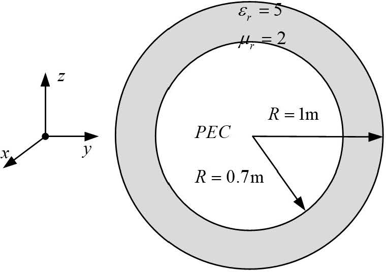
Figure 1: Two-layered sphere with a PEC core and a dielectric shell.

We have used two mesh structures to compare the accuracy and the convergence behavior. In case 1, the PEC surface and the dielectric part are meshed into 1320 triangles and 1946 tetrahedrons, respectively. The average length of the triangles is about $0.01{\lambda }_0$, ${\lambda }_0$ is the wavelength in free space. The average length of tetrahedrons is about $0.0763{\lambda }_D$, ${\lambda }_D$ is the wavelength in the interior region of dielectric part. The mesh structure generates 1980 RWGs, 3543 SWGs, and 698 HSWGs. Hence, the dimension of the impedance matrix is 10462$\times$10462. The mesh in case 2 is generated based on the mesh of case 1. From the meshes in case 1, we have selected the 162 triangles and 244 tetrahedrons in the region $x\ge 0$, $y\ge 0$, and $z\le 0$ for local refinement. By adding 3 additional nodes at the middle of the 3 edges of the triangle, each selected triangle is divided into 4 small triangles. Similarly, by adding 6 additional nodes at the middle of the 6 edges of the tetrahedron, each selected tetrahedron is divided into 8 small tetrahedrons. Hence, the refined meshes generate 2664 RWGs, 6692 SWGs, 962 HSWGs, 30 MBRWGs, and 54 MBSWGs in total. The dimension of the impedance matrix is changed to 18110$\times$18110.

To reduce the number of iterations, the four preconditioners, discussed in Section II, are applied. All the preconditioners can greatly accelerate the convergence of the GMRES iteration solver under nearly the same accuracy. The Bi-RCSs, obtained for the two mesh structures, are compared with those obtained by Mie series, as illustrated in Fig. 2. The relative error is -17.65 dB in case 1 and -25.05 dB in case 2. Moreover, we have applied four BDPs in case 2.

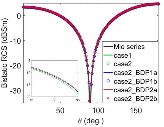
Figure 2: Bistatic RCSs for case 1, case 2, and case 2 with two BDPs, Mie series.

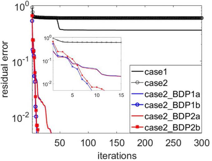
Figure 3: Iteration convergencies for different methods.

The relative error stays the same when different BDPs are applied. The iteration property and singular values of the impedance matrix in different cases are illustrated in Figs. 3 and 4, respectively. The condition numbers of case 2 with or without different BDPs and numbers of iterations to achieve a residual error of 0.005 are listed in Table 1. Obviously, the singular values are more clustered and the number of iterations is smaller after application of preconditioners [16][17].

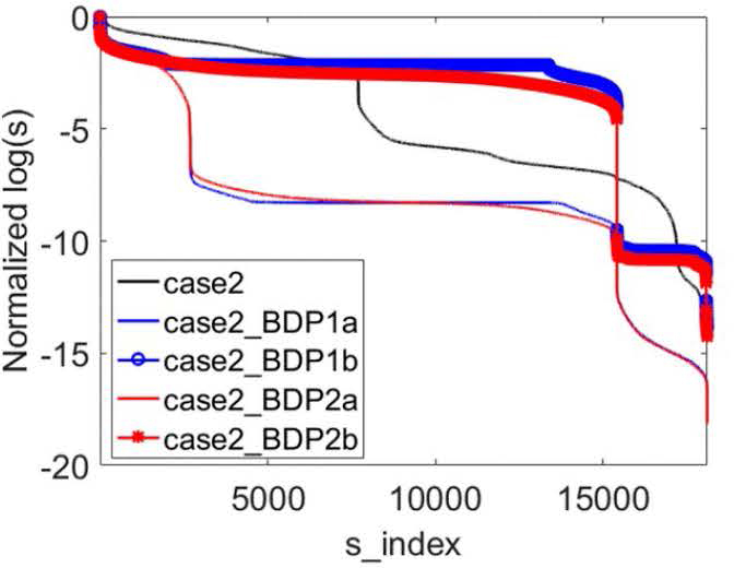
Figure 4: The s values of SVD for different methods.

Table 1: Condition numbers and numbers of iterations

Case 2	Condition Number	Number of Iterations
without BDP	$1.438\times {10}^{13}$	/
with BDP1a	$1.356\times {10}^{18}$	35
with BDP1b	$7.250\times {10}^{13}$	9
with BDP2a	$1.356\times {10}^{18}$	35
with BDP2b	$1.842\times {10}^{14}$	12

The second example is used to show the effect of local refinement for different materials. We consider a PEC cuboid, surrounded by two different materials and illuminated by a plane wave with frequency of 260 MHz, as shown in Fig. 5. The lengths of PEC cuboid along x, y, and z axis are 0.6 m, 0.1 m, and 0.1 m, respectively. The thickness of dielectric shell is 0.05 m. It consists of two kinds of materials. The dielectric in region 1 is anisotropic materials, with parameters of:

$${\overline{\epsilon }}_{r1}=\left[\begin{array}{ccc}\hfill 8+0.2j\hfill & \hfill -0.4j\hfill & \hfill 0\hfill \\ \hfill 0.4j\hfill & \hfill 8+0.2j\hfill & \hfill 0\hfill \\ \hfill 0\hfill & \hfill 0\hfill & \hfill 8-0.1j\hfill \end{array}\right],$$

${\mu }_{r1}=2$. The parameters of region 2 are ${\epsilon }_{r2}=2$, ${\mu }_{r2}=1.5$. The wavelengths in the dielectric part are labeled as ${\lambda }_n$, where $n=1,2$ for different regions.

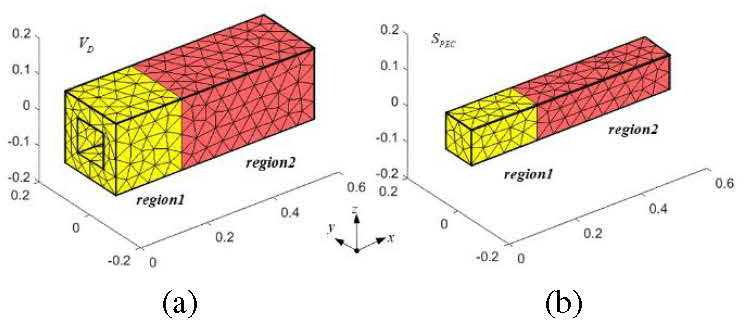
Figure 5: Model of the cuboid scatterer divided in w regions: (a) dielectric part and (b) PEC part.

Firstly, we generate a fine mesh structure as a base for comparison. The surface of the PEC part is divided into 360 triangles, and the dielectric part is divided into 2462 tetrahedrons. The fine mesh structure generates 4449 SWGs, 950 HSWGs, and 540 RWGs. The dimension of the impedance matrix is 11338$\times$11338. The average lengths are 0.036${\lambda }_0$ for the PEC part, 0.19${\lambda }_1$ and 0.089${\lambda }_2$ for the dielectric part.

Secondly, we generate a coarse mesh structure as the base for local refinement, where the surface of the PEC part is divided into 104 triangles, and the dielectric part is divided into 402 tetrahedrons. The coarse mesh structure generates 658 SWGs, 292 HSWGs, and 156 RWGs. The dimension of the impedance matrix is 2056$\times$2056. The average lengths are 0.066${\lambda }_0$ for the PEC part, 0.37${\lambda }_1$ and 0.16${\lambda }_2$ for the dielectric part.

Thirdly, based on the coarse mesh structure, progressive local refinements are considered to show the effect of different local refinement strategies. The refining approach for the selected part of meshes is the same as that in the first example.

In case 1, we only select the triangles/tetrahedrons in region 1 of PEC/dielectric part for local refinement, generating 2326 SWGs, 592 HSWGs, 12 MBSWGs, 312 RWGs, and 4 MBRWGs. The dimension of the impedance matrix is 6176$\times$6176.

Case 2 is based on case 1. We find the 4 triangles on the PEC surface in region 2 that have one side locating on the bordering line with region 1, and then add them as additional region for local refinement. The numbers of RWGs, MBRWGs, and the dimension of the impedance matrix are changed to 324, 8, and 6192$\times$6192, respectively.

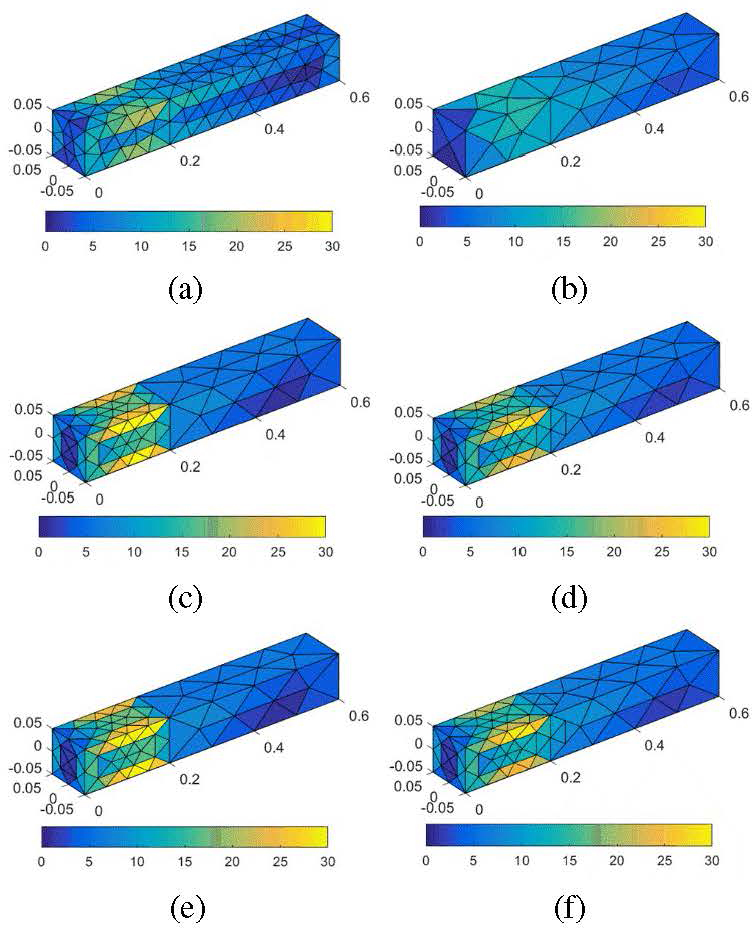
Figure 6: The surface currents of different cases (unit: mA/m): (a) fine case, (b) coarse case, and (c-f) case 1-4.

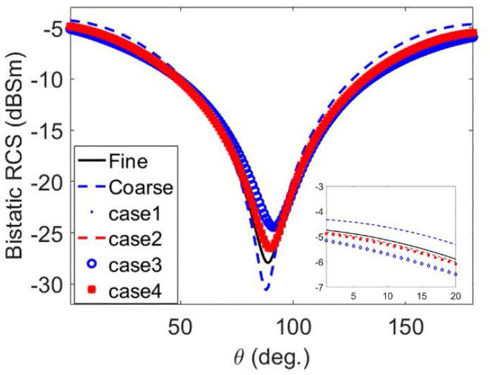
Figure 7: The results of bistatic RCSs of different cases in xoz plane.

Case 3 is also based on case 1. We find the 50 tetrahedrons in region 1 and region 3 of dielectric part that have a surface locating at the interface with region 2, then we add them for local refinement. The numbers of SWGs, HSWGs, MBSWGs, and the dimension of the impedance matrix are changed to 2446, 628, 24, and 6512$\times$6512, respectively.

In case 4, both of the additional meshes in case 2 and case 3 are selected for local refinement. The dimension of the impedance matrix is changed to 6528$\times$6528.

Obviously, the local refinement in case 1 has abrupt variation in mesh sizes in different material regions; in case 2, a transition region on the PEC surface is added; in case 3, a transition region in the dielectric region is added; and in case 4, both the transition regions are added. This is to show the effect of the different local refining strategies.

The results of the surface current on the PEC part and the Bi-RCSs of the object in the xoz plane in different cases are shown in Figs. 6 and 7, respectively. The relative errors of Bi-RCSs of the coarse mesh and cases 1-4 are -24.47 dB, -21.44 dB, -30.31 dB, -20.52 dB, and -28.61 dB compared with the Bi-RCSs of the fine mesh as a reference result.

It can be seen that surface current on the PEC surface is greatly affected by the discontinuity between different materials where there is no transition area on the surface of the PEC object. The local refinement in coarse meshes improves the Bi-RCSs result. Hence, the MBSWGs and MBRWGs can be applied for hybrid PEC and dielectric structures, especially when local refinement is needed.

IV. CONCLUSION

MB-RWGs can be applied for solving SIEs, and MB-SWGs can be applied for solving VIEs. Both have nearly the same accuracy as that of using traditional RWGs and SWGs [3][7]. In this paper, it is demonstrated that MB-RWG and MB-SWG can also be applied for solving SVIEs in hybrid systems even consisting of inhomogeneous and anisotropic materials.

Although MB-RWGs and MB-SWGs are flexible for local refinement, numerical examples show that, when performing local refinement among different types of materials, it would be better to refine the regions in a progressive way so that the scale of the mesh structures between neighboring elements is not toodifferent.

ACKNOWLEDGMENT

This work was supported by the National Science Foundation of China under Grant 62188102.

REFERENCES

[1] S. M. Rao, D. R. Wilton, and A. W. Glisson, “Electromagnetic scattering by surfaces of arbitrary shape,” IEEE Trans. Antennas Propagat., vol. 30, no. 3, pp. 409-418, 1982.

[2] P. Yla-Oijala and M. Taskinen, “Well-conditioned Müller formulation for electromagnetic scattering by dielectric objects,” IEEE Trans. Antennas Propagat., vol. 53, no. 10, pp. 3316-3323, Oct.2005.

[3] S. Huang, G. Xiao, Y. Hu, R. Liu, and J. Mao, “Multibranch Rao-Wilton-Glisson basis functions for electromagnetic scattering problems,” IEEE Trans. Antennas Propagat., vol. 69, no. 10, pp. 6624-6634, Oct. 2021.

[4] F. P. Andriulli, F. Vipiana, and G. Vecchi, “Hierarchical bases for nonhierarchic 3-D triangular meshes,” IEEE Trans. Antennas Propagat., vol. 56, no. 8, pp. 2288-2297, Aug. 2008.

[5] D. H. Schaubert, D. R. Wilton, and A. W. Glisson, “A tetrahedral modeling method for electromagnetic scattering by arbitrarily shaped inhomogeneous dielectric bodies,” IEEE Trans. Antennas Propagat., vol. 32, no. 1, pp. 77-85, Apr.1984.

[6] L. M. Zhang and X. Q. Sheng, “Solving volume electric current integral equation with full- and half-SWG functions,” IEEE Antennas and Wirel. Propaga. Lett., vol. 14, pp. 682-685, 2015.

[7] R. Liu, G. Xiao, S. Huang, and Y. Hu, “Multibranch Schaubert-Wilton-Glisson basis functions for electromagnetic scattering problem,” IEEE Trans. Antennas Propagat., vol. 70, no. 4, pp. 3100-3105, Apr. 2022.

[8] R. R. Chang, K. Chen, J. Wei, and M. S. Tong, “Reducing volume integrals to line integrals for some functions associated with Schaubert-Wilton-Glisson basis functions,” IEEE Trans. Antennas Propagat., vol. 69, no. 5, pp. 3033-3038, May 2021.

[9] C. C. Lu and W. C. Chew, “A coupled surface-volume integral equation approach for the calculation of electromagnetic scattering from composite metallic and material targets,” IEEE Trans. Antennas Propagat., vol. 48, no. 12, pp. 1866-1868, Dec. 2000.

[10] Q. M. Cai, Y. W. Zhao, W. F. Huang, Y. T. Zheng, Z. P. Zhang, Z. P. Nie, and Q. H. Liu, “Volume surface integral equation method based on higher order hierarchical vector basis functions for EM scattering and radiation from composite metallic and dielectric structures,” IEEE Trans. Antennas Propagat., vol. 64, no. 12, pp. 5359-5372, Dec. 2016.

[11] A. C. Yucel, L. J. Gomez, and E. Michielssen, “Internally combined volume-surface integral equation for EM analysis of inhomogeneous negative permittivity plasma scatterers,” IEEE Trans. Antennas Propagat., vol. 66, no. 4, pp. 1903-1913, Apr. 2018.

[12] B. J. Ward, “Hybrid surface electric field volume magnetic field integral equations for electromagnetic analysis of heterogeneous dielectric bodies with embedded electrically conducting structures,” IEEE Trans. Antennas Propagat., vol. 69, no. 3, pp. 1545-1552, Mar. 2021.

[13] W. D. Li, W. Hong, and H. X. Zhou, “An IE-ODDM-MLFMA scheme with DILU preconditioner for analysis of electromagnetic scattering from large complex objects,” IEEE Trans. Antennas Propagat., vol. 56, no. 5, pp. 1368-1380, May 2008.

[14] B. Kong, X. W. Huang, and X. Q. Sheng, “A discontinuous Galerkin surface integral solution for scattering from homogeneous objects with high dielectric constant,” IEEE Trans. Antennas Propagat., vol. 68, no. 1, pp. 598-603, Jan.2020.

[15] S. Z. Gu, L. Zhang, D. M. Yu, K. W. Xu, L. M. Si, and X. M. Pan, “On preconditioners of the FFT-JVIE for inhomogeneous dielectric objects,” IEEE Trans. Antennas Propagat., vol. 71, no. 6, pp. 5493-5497, June 2023.

[16] S. B. Adrian, A. Dely, D. Consoli, A. Merlini, and F. P. Andriulli, “Electromagnetic integral equations: Insights in conditioning and preconditioning,” IEEE Open Journal of Antennas and Propagation, vol. 2, pp. 1143-1174, Dec. 2021.

[17] X. Antoine and M. Darbas, “An introduction to operator preconditioning for the fast iterative integral equation solution of time-harmonic scattering problems,” Multiscale Sci. Eng., vol. 3, pp. 1-35, Feb. 2021.

BIOGRAPHIES

Rui Liu received B.S. degree from Shanghai Jiao Tong University, Shanghai, China, in 2017. He is currently pursuing Ph.D. degree in electronic engineering in Shanghai Jiao Tong University. His research interests include computational electromagnetics and inverse scattering problems.

Gaobiao Xiao received the B.S. degree from Huazhong University of Science and Technology, Wuhan, China, in 1988, M.S. degree from the National University of Defense Technology, Changsha, China, in 1991, and Ph.D. degree from Chiba University, Chiba, Japan, in 2002.

He has been a faculty member since 2004 in the Department of Electronic Engineering, Shanghai Jiao Tong University, Shanghai, China. His research interests are computational electromagnetics, coupled thermo-electromagnetic analysis, microwave filter designs, fiber-optic filter designs, phased array antennas, and inverse scattering problems.

Yuyang Hu received B.S. degree in telecommunications engineering from Xidian University, Xi’an, China, in 2018. He is currently pursuing Ph.D. degree with the State Key Laboratory of Radio Frequency Heterogeneous Integration, Shanghai Jiao Tong University, Shanghai. His current research interests include computational electromagnetics and its application in scattering and radiation problems.

ACES JOURNAL, Vol. 39, No. 2, 108–114
doi: 10.13052/2024.ACES.J.390203
© 2024 River Publishers

ABSTRACT

I. INTRODUCTION

II. SVIES FORMULATION

III. NUMERICAL EXAMPLES

IV. CONCLUSION

ACKNOWLEDGMENT

REFERENCES

BIOGRAPHIES