A Lossy Coated Thin Wire Model Based on the Unconditionally Stable Associated Hermite FDTD Method

Yi-Ru Zheng${}^{\text{1}}$, Sun Zheng${}^{\text{2}}$, Chen Chao${}^{\text{1}}$, Zheng-Yu Huang${}^{\text{1}}$, and Xin-Ran Chen${}^{\text{1}}$

¹Collage of Electronic and Information Engineering
Nanjing University of Aeronautics and Astronautics, Nanjing, 211106, China
zhengyiru0719@163.com, chenchao19991201@outlook.com, huangzynj@163.com, 790930183@qq.com

²Army Engineering University of PLA
Nanjing, 210007, China
sunzheng08005405@sina.com

Submitted On: June 30, 2023; Accepted On: July 1, 2025

ABSTRACT

This paper presents a lossy coated thin wire model based on the unconditionally stable (US) associated Hermite finite-difference time-domain (AH FDTD) method. The normal electric field discontinuity between lossy coated and surrounding media is corrected as the time-domain boundary condition. The coefficient matrix equation of lossy coated thin wires in AH domain is deduced by the static field model of infinite thin wires and the Faraday’s law contour-path formulation, finally the thin wires with lossy coated is modeled. Three examples of dipole antenna, five-element Yagi antenna and square antenna are used to verify the accuracy and high efficiency of the lossy coated thin wire model. The results show that the model can maintain the relative error of less than $-26$ dB and reduce computation time compared with the traditional FDTD method.

Index Terms: Associated Hermite (AH), Faraday’s law contour-path formulation, finite-different time-domain (FDTD), lossy coated thin wires, unconditionally stable (US).

I. INTRODUCTION

The lossy coated thin wires are widely used in communication circuit, underground detection, antenna system and other fields [1, 2]. The finite-difference time-domain (FDTD) method is a common electromagnetic calculation method. If this method is used to model thin wires, there will be a problem of long calculation time and large resource consumption [3, 4]. To avoid this problem, Holland and Simpson presented thin wires formalism based on I-Q the auxiliary differential equation [5].Railton et al. proposed two thin wire models using a weighted residual approach and modifying material parameters [6, 7]. Umashankar proposed thin wires model based on Faraday’s law contour-path formulation [8]. Ruddle et al. proposed and improved transmission line matrix (TLM) thin wires model [9].

Some unconditionally stable (US) FDTD methods can significantly reduce the resource utilization and improve the computational efficiency compared with the traditional FDTD methods. And they are not restricted by the Courant-Friedrichs-Lewy (CFL) condition. Shibayama et al. proposed and reviewed locally one-dimensional (LOD) FDTD [10]. Sun and Trueman proposed and applied Crank-Nicolson (CN) FDTD [11]. Chung et al. presented Laguerre FDTD [12]. Li et al. proposed Chebyshev (CS) FDTD [13]. Lee and Fornberg proposed split-step (SS) FDTD [14]. Associated Hermite (AH) FDTD is a US FDTD method proposed in 2014. The algorithm uses the Hermite orthogonal basis function to expand and reconstruct the electromagnetic field of the time domain in the Maxwell’s equation. It solves the coefficient matrix equation of three-dimensional AH FDTD in parallel according to different orders of Hermite orthogonal basis, and finally is applied to the electromagnetic calculation [15, 16].

In this paper, a lossy coated thin wire model based on the US AH FDTD method is proposed. First, the lossy coated thin wires algorithm in traditional FDTD is deduced based on the lossy media approximate boundary conditions, the static field model of infinite thin wires and the Faraday’s law contour-path formulation. Then, according to the modified electric field component, the lossy coated thin wires algorithm with AH FDTD is deduced. By using three examples of dipole antenna, five-element Yagi antenna and square antenna, the accuracy and efficiency of the algorithm are compared with the traditional FDTD method.

II. LOSSY COATED THIN WIRES MODEL BASED ON TRADITIONAL FDTD

The lossy coated thin wires consists of the ideal conductor with the inner radius of $r_0$ and the lossy coated with the outer radius of $r_c$. When using the Faraday’s law contour-path formulation to model the lossy coated thin wires in FDTD, the integral path and area in the equation include the lossy coated thin wires and the surrounding media, as shown in Fig. 1. Due to the discontinuity of the vertical electric field at the interface between the lossy coated and the surrounding media, it is necessary to derive the relationship between the electric fields on both sides first.

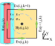
Figure 1: Lossy coated thin wires model.

Assuming that the materials involved in this paper are linear and isotropic. In the time domain, the electric flux density of lossy media with the relative permittivity ${\epsilon }_r$ and the conductivity $\sigma$ is defined as [17]:

$D(t)={\epsilon }_r{\epsilon }_{0}E(t)+{\displaystyle {\int }_0^t}E(t-\tau )\chi (\tau )d\tau ,$

(1)

where ${\epsilon }_0$ is the permittivity of free space and $\chi (\tau )$ is the electric susceptibility.

Equation (1) can be written as equation (II.) by time domain discretization ($t=n\mathrm{\Delta }t$).

$D(t)$	$=D(n\mathrm{\Delta }t)$
$=D^n={\epsilon }_r{\epsilon }_0{E}^n+{\displaystyle {\int }_0^{n\mathrm{\Delta }t}}E(n\mathrm{\Delta }t-\tau )\chi (\tau )d\tau .$	(2)

The complex permittivity in the frequency domain has the following form:

$\epsilon (\omega )={\epsilon }_r{\epsilon }_0+{\displaystyle \frac{\sigma }{j\omega }},$

(3)

where $\sigma$ is the conductivity of the media. It can be seen that the electric susceptibility is $\chi (\omega )=\frac{\sigma }{j\omega }$ in the frequency domain.

By using the Fourier inverse transform and substituting the time domain result of $\chi (\omega )$ into equation (II.), equation (II.) can be obtained as [18]:

$D^n$	$={\epsilon }_r{\epsilon }_0{E}^n+{\displaystyle \frac{\sigma \mathrm{\Delta }t}{2}}{\displaystyle \sum _{m=0}^{n-1}}{E}^{n-m}$
$=({\epsilon }_r{\epsilon }_0+{\displaystyle \frac{\sigma \mathrm{\Delta }t}{2}})E^n+{\displaystyle \frac{\sigma \mathrm{\Delta }t}{2}}{\displaystyle \sum _{m=1}^{n-1}}{E}^{n-m}.$	(4)

The boundary condition determines that the electric flux density perpendicular to the boundary is continuous. Using equation (II.), the electric field relationship perpendicular to the boundary ${\rho }_{is}$ of the two lossy materials (cable coating and surrounding media) is obtained as:

$E_s^n\cong K_{is}{E}_i^n+L_{is}{T}_{ss}^n,$

(5)

where

$T_{ss}^n$	$={\displaystyle \sum _{m=1}^{n-1}}{M}_{ss}^{m-1}{E}_i^{n-m},$	(6)
$K_{is}$	$={\displaystyle \frac{{\epsilon }_i{\epsilon }_0+{\sigma }_i\mathrm{\Delta }t/2}{{\epsilon }_s{\epsilon }_0+{\sigma }_s\mathrm{\Delta }t/2}},$	(7)
$L_{is}$	$={\displaystyle \frac{({\sigma }_i-{\sigma }_s{K}_{is})\mathrm{\Delta }t/2}{{\epsilon }_s{\epsilon }_0+{\sigma }_s\mathrm{\Delta }t/2}},$	(8)
$M_{ss}$	$={\displaystyle \frac{{\epsilon }_s{\epsilon }_0}{{\epsilon }_s{\epsilon }_0+{\sigma }_s\mathrm{\Delta }t/2}}.$	(9)

The subscripts $i$ and $s$ are the same as the areas marked in Fig. 1, representing the cable coating and the surrounding media respectively.

By approximating equation (5) and ignoring the higher order term $L_{is}{T}_{ss}^n$, the following equation can be obtained:

$E_s^n\cong K_{is}{E}_i^n={\displaystyle \frac{{\epsilon }_i{\epsilon }_0+{\sigma }_i\mathrm{\Delta }t/2}{{\epsilon }_s{\epsilon }_0+{\sigma }_s\mathrm{\Delta }t/2}}{E}_i^n.$

(10)

Thus, a constant $K_{is}$ is obtained to establish the electric field relationship between the lossy coated and the surrounding media.

Faraday’s law given in integral form as equation (11) can be applied on the enclosed surface shown in Fig. 1 to establish the relation between $H_y(i,j,k)$ and the electric field components located on the boundaries of the enclosed surface.

${\displaystyle {\oint }_L}\overrightarrow{E}\cdot \mathit{d}\overrightarrow{l}=-(\mu {\displaystyle {\int }_s}{\displaystyle \frac{\partial \overrightarrow{H}}{\partial t}}\cdot \mathit{d}\overrightarrow{s}+{\displaystyle {\int }_s}{\sigma }_m\overrightarrow{H}\cdot \mathit{d}\overrightarrow{s}).$

(11)

Finite radius thin wires can be modeled by near-field physical models. The variation of the fields (the near-scattered circumferential magnetic field component and the near-scattered radial electric field component) around the thin wires is assumed to be a function of $1/\rho$, as in equation (12). $\rho$ represents the distance to the field position from the thin-wire axis. The tangential electric field component inside the ideal conductor is set to zero.

$E_{\rho }(\rho ),H_{\varphi }(\rho )\propto {\displaystyle \frac{1}{\rho }}.$

(12)

When $r_0\le r_c\le \frac{\mathrm{\Delta }x}{2}$, the $E_x(\rho )$ can be obtained:

$E_x(\rho )|{}_{r_0\le \rho \le r_c,j,k}$	$={\displaystyle \frac{1}{K_{is}}}{\displaystyle \frac{E_x(i,j,k)\mathrm{\Delta }x}{2\rho }},$
$E_x(\rho )|{}_{r_c\le \rho \le \mathrm{\Delta }x,j,k}$	$={\displaystyle \frac{E_x(i,j,k)\mathrm{\Delta }x}{2\rho }},$
$E_x(\rho )|{}_{r_0\le \rho \le r_c,j,k+1}$	$={\displaystyle \frac{1}{K_{is}}}{\displaystyle \frac{E_x(i,j,k+1)\mathrm{\Delta }x}{2\rho }},$
$E_x(\rho )|{}_{r_c\le \rho \le \mathrm{\Delta }x,j,k+1}$	$={\displaystyle \frac{E_x(i,j,k+1)\mathrm{\Delta }x}{2\rho }}.$	(13)

Applying the above results to equation (11) and then simplifying, the lossy coated thin wires model for traditional FDTD are derived as:

$H_y^{n+\frac{1}{2}}(i,j,k)=$	$H_y^{n-\frac{1}{2}}(i,j,k)$
$+p_x{\displaystyle \frac{\mathrm{\Delta }t}{\mu \mathrm{\Delta }x}}$	$(E_z^n(i+1,j,k)-E_z^n(i,j,k))$
$+q_x{\displaystyle \frac{\mathrm{\Delta }t}{\mu \mathrm{\Delta }z}}$	$(E_x^n(i,j,k+1)-E_x^n(i,j,k)),$	(14)
$p_{\xi }={\displaystyle \frac{2}{\ln (\frac{{\mathrm{\Delta }}_{\xi }}{a})}}$	$,q_{\xi }={\displaystyle \frac{\left(\frac{\ln \left(\frac{r_c}{r_0}\right)}{K_{is}}+\ln \left(\frac{{\mathrm{\Delta }}_{\xi }}{r_c}\right)\right)}{\ln \left(\frac{{\mathrm{\Delta }}_{\xi }}{r_0}\right)}},$	(15)

where $p_{\xi }$ and $q_{\xi }$ are parameters that need to be modified. The permeability of the lossy coated is equal to that of surrounding media, that is $\mu$. And the effect of magnetic conductivity ${\sigma }_m$ is not considered. $\xi$ can be in the $x$, $y$ or $z$ direction.

Similarly, the update equation of the magnetic field component $H_y(i-1,j,k)$, $H_x(i,j,k)$ and $H_x(i,j-1,k)$ can be deduced.

III. LOSSY COATED THIN WIRES MODEL BASED ON AH FDTD

The coefficient matrix equation for lossy coated thin wires in AH domain will be derived below. The AH FDTD equations for Maxwell’s equations in lossy materials are as follows [19]:

${{\alpha }_{x(i,j,k)}^e{E}_x|}_{i,j,k}={\alpha }_{Sey(i,j,k)}^{-1}{\displaystyle \frac{({H_z|}_{i,j,k}-{H_z|}_{i,j-1,k})}{\mathrm{\Delta }{\overline{y}}_j}}$
$-{\alpha }_{Sez(i,j,k)}^{-1}{\displaystyle \frac{({H_y|}_{i,j,k}-{H_y|}_{i,j,k-1})}{\mathrm{\Delta }{\overline{z}}_k}}-{J_x|}_{i,j,k},$	(16)
${{\alpha }_{y(i,j,k)}^e{E}_y|}_{i,j,k}={\alpha }_{Sez(i,j,k)}^{-1}{\displaystyle \frac{({H_x|}_{i,j,k}-{H_x|}_{i,j,k-1})}{\mathrm{\Delta }{\overline{z}}_k}}$
$-{\alpha }_{Sex(i,j,k)}^{-1}{\displaystyle \frac{({H_z|}_{i,j,k}-{H_z|}_{i-1,j,k})}{\mathrm{\Delta }{\overline{x}}_i}}-{J_y|}_{i,j,k},$	(17)
${{\alpha }_{z(i,j,k)}^e{E}_z|}_{i,j,k}={\alpha }_{Sex(i,j,k)}^{-1}{\displaystyle \frac{({H_y|}_{i,j,k}-{H_y|}_{i-1,j,k})}{\mathrm{\Delta }{\overline{x}}_i}}$
$-{\alpha }_{Sey(i,j,k)}^{-1}{\displaystyle \frac{({H_x|}_{i,j,k}-{H_x|}_{i,j-1,k})}{\mathrm{\Delta }{\overline{y}}_j}}-{J_z|}_{i,j,k},$	(18)
${{\alpha }_{x(i,j,k)}^m{H}_x|}_{i,j,k}={\alpha }_{Smz(i,j,k)}^{-1}{\displaystyle \frac{({E_y|}_{i,j,k+1}-{E_y|}_{i,j,k})}{\mathrm{\Delta }{z}_k}}$
$-{\alpha }_{Smy(i,j,k)}^{-1}{\displaystyle \frac{({E_z|}_{i,j+1,k}-{E_z|}_{i,j,k})}{\mathrm{\Delta }{y}_j}}-{M_x|}_{i,j,k},$	(19)
${{\alpha }_{y(i,j,k)}^m{H}_y|}_{i,j,k}={\alpha }_{Smx(i,j,k)}^{-1}{\displaystyle \frac{({E_z|}_{i+1,j,k}-{E_z|}_{i,j,k})}{\mathrm{\Delta }{x}_i}}$
$-{\alpha }_{Smz(i,j,k)}^{-1}{\displaystyle \frac{({E_x|}_{i,j,k+1}-{E_x|}_{i,j,k})}{\mathrm{\Delta }{z}_k}}-{M_y|}_{i,j,k},$	(20)
${{\alpha }_{z(i,j,k)}^m{H}_z|}_{i,j,k}={\alpha }_{Smy(i,j,k)}^{-1}{\displaystyle \frac{({E_x|}_{i,j+1,k}-{E_x|}_{i,j,k})}{\mathrm{\Delta }{y}_j}}$
$-{\alpha }_{Smx(i,j,k)}^{-1}{\displaystyle \frac{({E_y|}_{i+1,j,k}-{E_y|}_{i,j,k})}{\mathrm{\Delta }{x}_i}}-{M_z|}_{i,j,k}.$	(21)

The intermediate variables of AH equation are given:

${\alpha }_{Se\xi (i,j,k)}$	$={{\kappa }_{e\xi }|}_{i,j,k}I+{{\sigma }_{pe\xi }|}_{i,j,k}{({{\eta }_{e\xi }|}_{i,j,k}I+\alpha {\epsilon }_0)}^{-1},$
${\alpha }_{Sm\xi (i,j,k)}$	$={{\kappa }_{m\xi }|}_{i,j,k}I+{{\sigma }_{pm\xi }|}_{i,j,k}{({{\eta }_{m\xi }|}_{i,j,k}I+\alpha {\mu }_0)}^{-1},$
${\alpha }_{\xi (i,j,k)}^e$	$={{\epsilon }_{\xi }|}_{i,j,k}\alpha +({{\sigma }_{\xi }^e|}_{i,j,k})I,$
${\alpha }_{\xi (i,j,k)}^m$	$={{\mu }_{\xi }|}_{i,j,k}\alpha +({{\sigma }_{\xi }^m|}_{i,j,k})I,$	(22)

where $\alpha$ is the AH differential transfer matrix. ${\epsilon }_{\xi }$ and ${\mu }_{\xi }$ are dielectric constants and permeability respectively.

Considering the lossy coated thin wires along the z-axis shown in Fig. 1, equation (II.) is migrated into the AH domain to obtain the correction equation (III.) for magnetic field ${H_y|}_{i,j,k}$.

${{\alpha }_{y(i,j,k)}^m{H}_y|}_{i,j,k}$	$=p_x{\alpha }_{Smx(i,j,k)}^{-1}{\displaystyle \frac{({E_z|}_{i+1,j,k}-{E_z|}_{i,j,k})}{\mathrm{\Delta }{x}_i}}$
$-q_x{\alpha }_{Smz(i,j,k)}^{-1}{\displaystyle \frac{({E_x|}_{i,j,k+1}-{E_x|}_{i,j,k})}{\mathrm{\Delta }{z}_k}}$
$-{M_y|}_{i,j,k}.$	(23)

Similarly, the modified equation of magnetic field ${H_y|}_{i-1,j,k}$, ${H_x|}_{i,j,k}$ and ${H_x|}_{i,j-1,k}$ can be obtained. In the three-dimensional AH domain, the electric field component needs to be modified for the lossy coated thin wires model. In Fig. 2, taking the positive side of the x-axis of lossy coated thin wires as an example, the following four kinds of electric field components need to be modified:

1. There are lossy coated thin wires above and below the electric field component, like ${E_x|}_{i,j,k}$. Equation (III.) shows that ${E_x|}_{i,j,k}$ is affected by ${H_y|}_{i,j,k}$, ${H_y|}_{i,j,k-1}$, ${H_z|}_{i,j,k}$ and ${H_z|}_{i,j-1,k}$. Because of the existence of the lossy coated thin wires model, ${H_y|}_{i,j,k}$ and ${H_y|}_{i,j,k-1}$ need to be modified. So the modified ${E_x|}_{i,j,k}$ update equation is equation (III.).

2. There are lossy coated thin wires below the electric field component, like ${E_x|}_{i,j,k+1}$. Equation (III.) shows that ${E_x|}_{i,j,k+1}$ is affected by ${H_y|}_{i,j,k+1}$, ${H_y|}_{i,j,k}$, ${H_z|}_{i,j,k+1}$ and ${H_z|}_{i,j-1,k+1}$. Similarly, ${H_y|}_{i,j,k}$ needs to be modified.

3. There are lossy coated thin wires above the electric field component, like ${E_x|}_{i,j,k-1}$. Equation (III.) shows that ${E_x|}_{i,j,k-1}$ is affected by ${H_y|}_{i,j,k-1}$, ${H_y|}_{i,j,k-2}$, ${H_z|}_{i,j,k-1}$ and ${H_z|}_{i,j-1,k-1}$. Similarly, ${H_y|}_{i,j,k-1}$ needs to be modified.

4. The electric field component is one grid away from the center of the lossy coated thin wires and the direction is along the thin wires, like ${E_z|}_{i+1,j,k}$, ${E_z|}_{i+1,j,k-1}$. Equation (18) shows that ${E_z|}_{i+1,j,k}$ is affected by ${H_y|}_{i+1,j,k}$, ${H_y|}_{i,j,k}$, ${H_x|}_{i+1,j,k}$ and ${H_x|}_{i+1,j-1,k}$. Similarly, ${H_y|}_{i,j,k}$ need to be modified. ${E_z|}_{i+1,j,k-1}$ is modified in the same way as ${E_z|}_{i+1,j,k}$.

${\alpha }_{Sey(i,j,k)}^{-1}{\alpha }_{z(i,j,k)}^{m-1}{\alpha }_{Smy(i,j,k)}^{-1}{\displaystyle \frac{{E_x|}_{i,j+1,k}-{E_x|}_{i,j,k}}{\mathrm{\Delta }{y}_j\mathrm{\Delta }{\overline{y}}_j}}+{\alpha }_{Sey(i,j,k)}^{-1}{\alpha }_{z(i,j-1,k)}^{m-1}{\alpha }_{Smy(i,j-1,k)}^{-1}{\displaystyle \frac{{E_x|}_{i,j-1,k}-{E_x|}_{i,j,k}}{\mathrm{\Delta }{y}_{j-1}\mathrm{\Delta }{\overline{y}}_j}}$
$+q_x{\alpha }_{Sez(i,j,k)}^{-1}{\alpha }_{y(i,j,k)}^{m-1}{\alpha }_{Smz(i,j,k)}^{-1}{\displaystyle \frac{{E_x|}_{i,j,k+1}-{E_x|}_{i,j,k}}{\mathrm{\Delta }{z}_k\mathrm{\Delta }{\overline{z}}_k}}+q_x{\alpha }_{Sez(i,j,k)}^{-1}{\alpha }_{y(i,j,k-1)}^{m-1}{\alpha }_{Smz(i,j,k-1)}^{-1}{\displaystyle \frac{{E_x|}_{i,j,k-1}-{E_x|}_{i,j,k}}{\mathrm{\Delta }{z}_{k-1}\mathrm{\Delta }{\overline{z}}_k}}$
$-{{\alpha }_{x(i,j,k)}^e{E}_x|}_{i,j,k}$
$+{\alpha }_{Sey(i,j,k)}^{-1}{\alpha }_{z(i,j,k)}^{m-1}{\alpha }_{Smx(i,j,k)}^{-1}{\displaystyle \frac{{E_y|}_{i,j,k}-{E_y|}_{i+1,j,k}}{\mathrm{\Delta }{x}_i\mathrm{\Delta }{\overline{y}}_j}}+{\alpha }_{Sey(i,j,k)}^{-1}{\alpha }_{z(i,j-1,k)}^{m-1}{\alpha }_{Smx(i,j-1,k)}^{-1}{\displaystyle \frac{{E_y|}_{i+1,j-1,k}-{E_y|}_{i,j-1,k}}{\mathrm{\Delta }{x}_i\mathrm{\Delta }{\overline{y}}_i}}$
$+p_x{\alpha }_{Sez(i,j,k)}^{-1}{\alpha }_{y(i,j,k)}^{m-1}{\alpha }_{Smx(i,j,k)}^{-1}{\displaystyle \frac{{E_z|}_{i,j,k}-{E_z|}_{i+1,j,k}}{\mathrm{\Delta }{x}_i\mathrm{\Delta }{\overline{z}}_k}}+p_x{\alpha }_{Sez(i,j,k)}^{-1}{\alpha }_{y(i,j,k-1)}^{m-1}{\alpha }_{Smx(i,j,k-1)}^{-1}{\displaystyle \frac{{E_z|}_{i+1,j,k-1}-{E_z|}_{i,j,k-1}}{\mathrm{\Delta }{x}_i\mathrm{\Delta }{\overline{z}}_k}}$
$={J_x|}_{i,j,k}-{\alpha }_{Sez(i,j,k)}^{-1}{\alpha }_{y(i,j,k)}^{m-1}{\displaystyle \frac{{M_y|}_{i,j,k}}{\mathrm{\Delta }{\overline{z}}_k}}+{\alpha }_{Sez(i,j,k)}^{-1}{\alpha }_{y(i,j,k-1)}^{m-1}{\displaystyle \frac{{M_y|}_{i,j,k-1}}{\mathrm{\Delta }{\overline{z}}_k}}$
$+{\alpha }_{Sey(i,j,k)}^{-1}{\alpha }_{z(i,j,k)}^{m-1}{\displaystyle \frac{{M_z|}_{i,j,k}}{\mathrm{\Delta }{\overline{y}}_j}}-{\alpha }_{Sey(i,j,k)}^{-1}{\alpha }_{z(i,j-1,k)}^{m-1}{\displaystyle \frac{{M_z|}_{i,j-1,k}}{\mathrm{\Delta }{\overline{y}}_j}}.$	(24)

Similarly, all electric field component modified equations can be obtained when the lossy coated thin wires follows any direction (x, y or z), and the modification is reflected in $p_{\xi }$ and $q_{\xi }$. So, the lossy coated thin wires model based on the three-dimensional AH FDTD method has been completed.

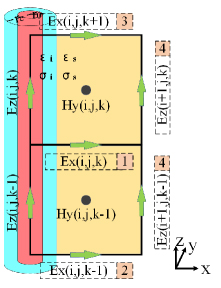
Figure 2: Modified electric field components.

IV. NUMERICAL ANALYSIS

A. Dipole antenna

A dipole antenna model is constructed using lossy coated thin wires. The uniform mesh size $\mathrm{\Delta }=0.25\times {10}^{-3}$ m, the total length of dipole antenna is 80$\mathrm{\Delta }$, the voltage source length of 2$\mathrm{\Delta }$, and the excitation waveform is $\exp (-{((t-2.81\times {10}^{-11})/(6.25\times {10}^{-12}))}^2)$, the resistance of source is 50 $\mathrm{\Omega }$. The radii of the thin wires are $r_0=\mathrm{\Delta }/10$ and $r_c=\mathrm{\Delta }/5$ respectively. The lossy coated and surrounding media are constructed from two common groups of materials: Teflon (${\epsilon }_i=$ 2.1 and ${\sigma }_i=$ 5 $\mu$S/m) and 5% wet soil (${\epsilon }_s=$ 5.0 and ${\sigma }_s=$ 17 mS/m), Alumina (${\epsilon }_i=$ 8.8 and ${\sigma }_i=$ 1.5 mS/m) and Air (${\epsilon }_s=$ 1 and ${\sigma }_s=$ 0). Figure 3 shows the sampling current at the center of the dipole antenna by the AH FDTD and the traditional FDTD.

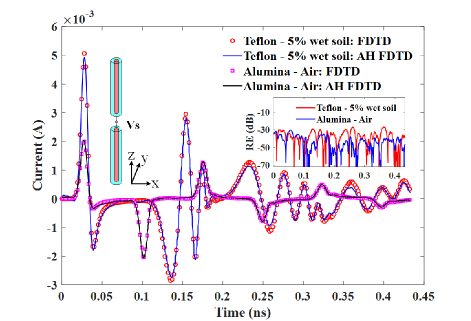
Figure 3: The sampling current at the center point.

The results show that the relative error of sampling current between conventional FDTD and AH FDTD can be about $-30$ dB when calculating the dipole antenna of different materials (${\epsilon }_i$, ${\sigma }_i$, ${\epsilon }_s$, ${\sigma }_s$).

For additional verification, a cosine-modulated Gaussian excitation source was employed with an extended time step. The FDTD and AH-FDTD results, as shown in Fig. 4, exhibit excellent agreement under the same conditions, consistent with theoretical predictions.

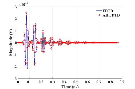
Figure 4: A cosine-modulated Gaussian excitation source was employed with an extended time step.

B. Yagi antenna

A five-element Yagi antenna is constructed with lossy coated thin wires. The uniform grid size $\mathrm{\Delta }=0.01$ m, reflector length $L_r=22\mathrm{\Delta }$, dipole length $L=20\mathrm{\Delta }$, three directors length $L_d=18\mathrm{\Delta }$, reflector-dipole spacing $S_r=8\mathrm{\Delta }$, and director-dipole spacing $S_d=10\mathrm{\Delta }$. Three lossy coated thin wires with the same material (Alumina) but different structural parameters are simulated: $r_0=\mathrm{\Delta }/10$, $r_c=\mathrm{\Delta }/5$, $r_0=\mathrm{\Delta }/50$, $r_c=\mathrm{\Delta }/25$, $r_0=\mathrm{\Delta }/50$, $r_c=\mathrm{\Delta }/10$. The excitation voltage source waveform is $100\times \exp (-{((t-3.60\times {10}^{-9})/(8.01\times {10}^{-10}))}^2)$, with a maximum frequence of 625 MHz. Figure 5 shows the far field radiation patterns (xy plane) of the Yagi antenna calculated by AH FDTD and traditional FDTD respectively, with the frequence of 625 MHz.

It can be seen that the results are well matched with traditional FDTD method, when calculating the far-field radiation pattern of the five-element Yagi antenna composed of wires with different structural parameters (radius of wires and coatings).

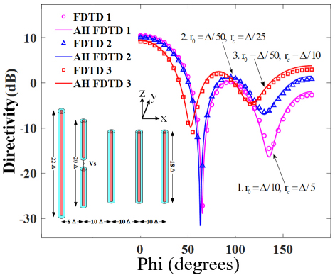
Figure 5: Radiation pattern in the xy plane cut.

C. Square antenna

A square antenna model is constructed using lossy coated thin wires. The uniform grid size $\mathrm{\Delta }=0.25$ m and antenna edge length is 8$\mathrm{\Delta }$. The thin wires structural parameters are $r_0=\mathrm{\Delta }/10$ and $r_c=\mathrm{\Delta }/5$. The lossy coated and the surrounding medium are constructed with Teflon and 5% wet soil respectively. The voltage source length is 2$\mathrm{\Delta }$, an internal resistance of 50 $\mathrm{\Omega }$. The maximum frequencies of the Gaussian pulse are 60 MHz, 40 MHz and 24 MHz. Figure 6 shows the sampled electric field $E_z$ at the center point of the square antenna calculated by AH FDTD and traditional FDTD respectively. Figure 7 shows the radiation pattern at a valid frequency.

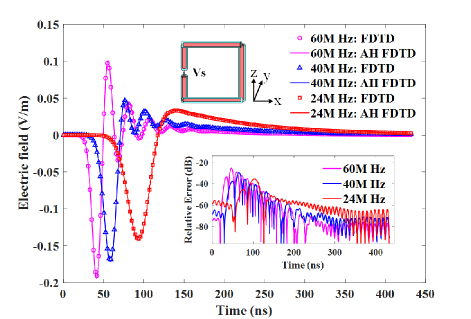
Figure 6: $E_z$ at the center point of the square antenna.

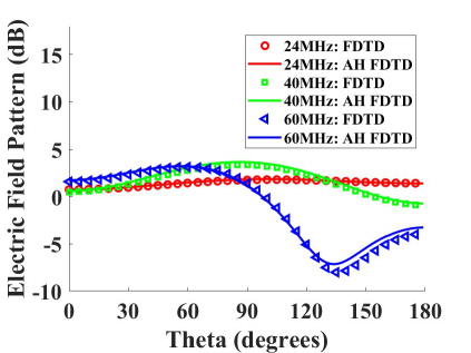
Figure 7: The radiation pattern at a valid frequency.

Table 1: Comparison of acceleration factors and relative errors between AH FDTD and FDTD

Frequency (MHz)	$t_{FDTD}$ (s)	$t_{AH}$ (s)	Acceleration Factors	($t_{FDTD}$/$t_{AH}$)	Relative Error(dB)
24	12	7	1.7	-35
12	18	7	2.6	-41
6	34	7	4.8	-44
4	41	7	5.9	-45
3	50	7	7.1	-46
2.4	60	7	8.6	-47

It can be seen that AH FDTD can maintain the relative error below $-26$ dB compared with traditional FDTD when calculating the electric field $E_z$ at the center point of the square antenna.

The calculation efficiency of the lossy coated thin wires model is presented below. The maximum frequencies of the excitation sources were set at 24 MHz, 12 MHz, 6 MHz, 4 MHz, 3 MHz and 2.4 MHz, and the time steps are 1000, 2000, 4000, 6000, 8000 and 10000 respectively. The AH FDTD method overcomes the conventional CFL time step constraint, leading to fundamentally different time step selection criteria compared to traditional explicit FDTD schemes. Table 1 shows the acceleration factors ($t_{FDTD}/t_{AH}$) and relative errors under different excitation sources. Since the lossy coated thin wires model can be parallel calculated according to different orders of Hermite orthogonal basis in AH domain, the simulation time can be greatly accelerated (1.7 to 8.6 times) while keeping the relative error below $-35$ dB.

V. CONCLUSION

This paper presents a lossy coated thin-wire model based on the unconditionally stable associated Hermite finite-difference time-domain (AH-FDTD) method. Validation tests on dipole antennas, five-element Yagi antennas, and square antennas confirm the model’s advantages. Compared to conventional FDTD methods, it achieves a relative error of less than -26 dB. The combination of the coated thin-wire model with the AH-FDTD method enhances the accuracy and computational efficiency of antenna simulations.

ACKNOWLEDGEMENT

This work was supported in part by National Key Laboratory Foundation of China under Grant JCKYS2023LD5, Aeronautical Science Foundation of China (Grant NO. 20240018052002), National Natural Science Foundation of China under Grant 61801217, Natural Science Foundation of Jiangsu Province under Grant BK20180422 and Funded by the National Key Laboratory on Electromagnetic Environmental Effects and Electro-optical Engineering (NO.61422062305).

REFERENCES

[1] T. Hertel and G. Smith, “The insulated linear antenna-revisited,” IEEE Transactions on Antennas and Propagation, vol. 48, no. 6, pp. 914–920, 2000.

[2] J. Willoughby and P. Lowell, “Development of loop aerial for submarine radio communication,” Phys. Rev, vol. 14, pp. 193–194, 1919.

[3] A. Taflove, S. C. Hagness, and M. Piket-May, “Computational electromagnetics: The finite-difference time-domain method,” The Electrical Engineering Handbook, vol. 3, pp. 629–670, 2005.

[4] J. Boonzaaier and C. Pistonius, “Finite-difference time-domain field approximations for thin wires with a lossy coating,” IEE Proceedings-Microwaves, Antennas and Propagation, vol. 141, no. 2, pp. 107–113, 1994.

[5] R. Holland and L. Simpson, “Finite-difference analysis of EMP coupling to thin struts and wires,” IEEE Transactions on Electromagnetic Compatibility, vol. EMC-23, no. 2, pp. 88–97, 1981.

[6] C. J. Railton, B. P. Koh, and I. J. Craddock, “The treatment of thin wires in the FDTD method using a weighted residuals approach,” IEEE Transactions on Antennas and Propagation, vol. 52, no. 11, pp. 2941–2949, 2004.

[7] C. J. Railton, D. L. Paul, I. J. Craddock, and G. S. Hilton, “The treatment of geometrically small structures in FDTD by the modification of assigned material parameters,” IEEE Transactions on Antennas and Propagation, vol. 53, no. 12, pp. 4129–4136, 2005.

[8] K. Umashankar, A. Taflove, and B. Beker, “Calculation and experimental validation of induced currents on coupled wires in an arbitrary shaped cavity,” IEEE Transactions on Antennas and Propagation, vol. 35, no. 11, pp. 1248–1257, 1987.

[9] A. Ruddle, D. Ward, R. Scaramuzza, and V. Trenkic, “Development of thin wire models in TLM,” in 1998 IEEE EMC Symposium. International Symposium on Electromagnetic Compatibility. Symposium Record (Cat. No. 98CH36253), vol. 1, pp. 196–201, 1998.

[10] J. Shibayama, M. Muraki, J. Yamauchi, and H. Nakano, “Efficient implicit FDTD algorithm based on locally one-dimensional scheme,” Electronics Letters, vol. 41, no. 19, p. 1, 2005.

[11] C. Sun and C. Trueman, “Unconditionally stable Crank-Nicolson scheme for solving two-dimensional Maxwell’s equations,” Electronics Letters, vol. 39, no. 7, pp. 595–597, 2003.

[12] Y.-S. Chung, T. K. Sarkar, B. H. Jung, and M. Salazar-Palma, “An unconditionally stable scheme for the finite-difference time-domain method,” IEEE Transactions on Microwave Theory and Techniques, vol. 51, no. 3, pp. 697–704, 2003.

[13] C. Li, Z.-Y. Huang, Z.-A. Chen, S. Zhu, A.-W. Yang, and Z.-J. Wang, “Unconditionally stable FDTD method based on Chebyshev polynomials—Chebyshev (CS) FDTD,” in 2021 International Applied Computational Electromagnetics Society (ACES-China) Symposium, pp. 1–2, 2021.

[14] J. Lee and B. Fornberg, “A split step approach for the 3-D Maxwell’s equations,” Journal of Computational and Applied Mathematics, vol. 158, no. 2, pp. 485–505, 2003.

[15] Z.-Y. Huang, L.-H. Shi, and B. Chen, “The 3-D unconditionally stable associated Hermite finite-difference time-domain method,” IEEE Transactions on Antennas and Propagation, vol. 68, no. 7, pp. 5534–5543, 2020.

[16] Z. Chen, Z. Huang, S. Liu, Q. Zeng, and R. E. V. Lorena, “The associated Hermite FDTD method with the thin-wire modeling in low-frequency cases,” IEEE Journal on Multiscale and Multiphysics Computational Techniques, vol. 7, pp. 56–60, 2022.

[17] R. Luebbers, F. P. Hunsberger, K. S. Kunz, R. B. Standler, and M. Schneider, “A frequency-dependent finite-difference time-domain formulation for dispersive materials,” IEEE Transactions on Electromagnetic Compatibility, vol. 32, no. 3, pp. 222–227, 1990.

[18] S.-Y. Hyun and S.-Y. Kim, “Thin-wire model using subcellular extensions in the finite-difference time-domain analysis of thin and lossy insulated cylindrical structures in lossy media,” IEEE Transactions on Electromagnetic Compatibility, vol. 51, no. 4, pp. 1009–1016, 2009.

[19] Z.-Y. Huang, L.-H. Shi, and B. Chen, “Efficient implementation for the AH FDTD method with iterative procedure and CFS-PML,” IEEE Transactions on Antennas and Propagation, vol. 65, no. 5, pp. 2728–2733, 2017.

BIOGRAPHIES

Yi-Ru Zheng was born in Hubei, China, in 2001. She received a B.D. degree from China Three Gorges University in 2023. She is currently working on her M.D. at Nanjing University of Aeronautics and Astronautics. Her research interests include EMC, FDTD, PINN.

Sun Zheng received the B.S. degree in Automatic control in 2009 from Southeast University, Jiangsu, China and Ph.D. degree in electrical engineering from PLA University of Science & Technology, Jiangsu, China, in 2014, respectively. He is currently working as a lecturer in the PLA Army Engineering University, with his main interests in computing electromagnetics and lightning protections.

Chen Chao was born in Anhui, China, in 1999. He received a B.D. from Shantou University, China in 2021. He is currently working on his M.D. at Nanjing University of Aeronautics and Astronautics. His research interests include EMC, FDTD.

Zheng-Yu Huang is an Associate Professor in the Department of Electronic and Information Engineering at Nanjing University of Aeronautics and Astronautics, China. He holds memberships in IEEE, IET, and ACES, and is a Senior Member of the Chinese Institute of Electronics. His research interests include computational electromagnetics, with a focus on fast algorithms, multi-physics modeling, and physics-informed machine learning methods. In 2014, he proposed the AH FDTD method, an efficient and unconditionally stable time-domain approach based on orthogonal expansion in time-domain (OETD), which demonstrates significant potential for multi-scale and multi-physics simulations. The method has been continuously improved through advances in wave excitation schemes, absorbing boundary conditions, iterative solvers, periodic structure analysis, dispersive media modeling, low-frequency analysis, and parallel computing techniques. He was recognized as a Young Scientific Talent by the Jiangsu Association for Science and Technology in 2019, and as a Young Scientist by ACES-China in 2021. He is the author of one research monograph “The Unconditionally Stable Associated Hermite FDTD Algorithm” (Science Press) and one textbook “Research Skills and Techniques for Electronics and Information Engineering” (Tsinghua University Press). He also serves as a reviewer for leading journals, including IEEE Transactions on Antennas and Propagation, IEEE Transactions on Microwave Theory and Techniques, IEEE Antennas and Wireless Propagation Letters, and the Applied Computational Electromagnetics Society Journal. He has served as a session chair and technical program committee member for major international conferences, such as ACES, ICCEM, PIERS, UCMMT, CSQRW, and APEMC.

Xin-Ran Chen was born in China. She received her B.E. degree from China University of Petroleum (East China) in 2024. She is currently pursuing her M.E. degree at Nanjing University of Aeronautics and Astronautics. Her research interests include EMC, FDTD.

ACES JOURNAL, Vol. 40, No. 7, 571–578
doi: 10.13052/2024.ACES.J.400701
© 2025 River Publishers